Recently I came across a machine learning algorithm called 'k-nearest neighbors' or 'kNN,' which is used as a predictive modeling tool. This algorithm uses data to build a model and then uses that model to predict the outcome.
kNN is new for me, and I gained most of my knowledge by reading these two tutorials; tutorial 1 and tutorial 2.
I will apply the kNN algorithm in the NHANES data set to predict diabetes.
Load 'tidyverse,' 'class,' and 'NHANES' packages.
library(tidyverse)
library(RNHANES)
library(class)
Import the dataset
DEMO_F = nhanes_load_data("DEMO_F", "2009-2010") %>%
  select(SEQN, RIDAGEYR)
BMX_F = nhanes_load_data("BMX_F", "2009-2010") %>%
  select(SEQN, BMXBMI, BMXWT)
HDL_F =  nhanes_load_data("HDL_F", "2009-2010") %>%
  select(SEQN, LBDHDD)
GLU_F = nhanes_load_data("GLU_F", "2009-2010") %>%
  select(SEQN, LBXGLU, LBXIN)
DIQ_F = nhanes_load_data("DIQ_F", "2009-2010") %>%
  select(SEQN, DIQ010)
Merge the data in one dataset and remove missing values.
dtx = left_join(DEMO_F, HDL_F) %>%
  left_join(GLU_F) %>%
  left_join(BMX_F) %>%
  left_join(DIQ_F)

dat = dtx %>%
  filter(!is.na(BMXBMI), !is.na(LBDHDD), !is.na(LBXGLU), !is.na(LBXIN),RIDAGEYR >= 40, DIQ010 %in% c(1, 2)) %>%
  transmute(SEQN, Age = RIDAGEYR, BMI = BMXBMI, Cholest = LBDHDD, Glucose = LBXGLU, Insuline = LBXIN, Weight = BMXWT, Diabetes = DIQ010) %>%
  mutate(Diabetes = recode_factor(Diabetes,
                           `1` = "Yes",
                           `2` = "No"))
Explore data
Now that I have the dataset, I will evaluate the correlation between two variables (glucose and weight) using the 'ggplot2' package.
ggplot(dat, aes(Glucose, Weight, color = Diabetes)) +
  geom_point(alpha = 0.7, size = 2)
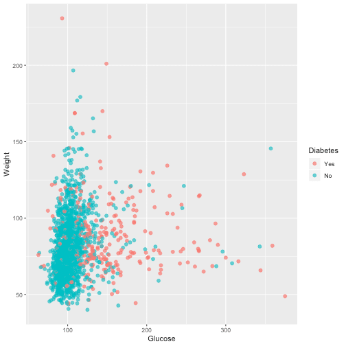
From the graph, it is evident that the higher the level of blood glucose more diabetes events we have.
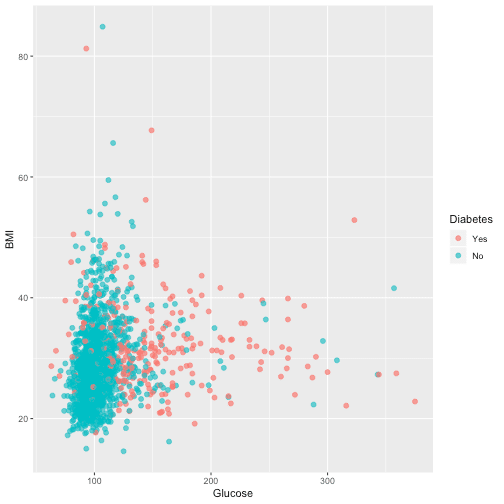
Another relationship I want to assess is Blood glucose and BMI:
ggplot(dat, aes(Glucose, BMI, color = Diabetes)) +
  geom_point(alpha = 0.7, size = 2)
Prepare the data set
To proceed with preparing the data, I would like to get more information regarding all variables, and I use 'summary' function:
summary(dat)
##       SEQN            Age             BMI           Cholest          Glucose
##  Min.   :51645   Min.   :40.00   Min.   :14.59   Min.   : 19.00   Min.   : 63
##  1st Qu.:54366   1st Qu.:48.00   1st Qu.:24.96   1st Qu.: 43.00   1st Qu.: 95
##  Median :57096   Median :59.00   Median :28.31   Median : 52.00   Median :102
##  Mean   :56983   Mean   :59.23   Mean   :29.36   Mean   : 54.66   Mean   :111
##  3rd Qu.:59593   3rd Qu.:70.00   3rd Qu.:32.62   3rd Qu.: 64.00   3rd Qu.:114
##  Max.   :62158   Max.   :80.00   Max.   :84.87   Max.   :144.00   Max.   :375
##     Insuline           Weight       Diabetes
##  Min.   :  0.880   Min.   : 40.10   Yes: 286
##  1st Qu.:  7.008   1st Qu.: 66.90   No :1486
##  Median : 11.405   Median : 78.15
##  Mean   : 15.101   Mean   : 81.73
##  3rd Qu.: 17.995   3rd Qu.: 92.92
##  Max.   :320.220   Max.   :230.70
Here I see a different range of values in my variables; therefore, I will normalize my numeric variables (the predictors) to prepare them for using in the kNN algorithm. I create the normalize function and then apply it to the predictor variables as below:
normalize <- function (i) {
  (i - min(i))/(max(i) - min(i))
}

norm_dat <- dat %>%
  select(Age, BMI, Cholest, Glucose, Insuline, Weight) %>%
  lapply(., normalize) %>%
  as.data.frame()
All the new values are within the range of 0 and 1.
summary(norm_dat)
##       Age              BMI            Cholest          Glucose          Insuline
##  Min.   :0.0000   Min.   :0.0000   Min.   :0.0000   Min.   :0.0000   Min.   :0.00000
##  1st Qu.:0.2000   1st Qu.:0.1476   1st Qu.:0.1920   1st Qu.:0.1026   1st Qu.:0.01919
##  Median :0.4750   Median :0.1952   Median :0.2640   Median :0.1250   Median :0.03296
##  Mean   :0.4807   Mean   :0.2102   Mean   :0.2853   Mean   :0.1539   Mean   :0.04453
##  3rd Qu.:0.7500   3rd Qu.:0.2565   3rd Qu.:0.3600   3rd Qu.:0.1635   3rd Qu.:0.05359
##  Max.   :1.0000   Max.   :1.0000   Max.   :1.0000   Max.   :1.0000   Max.   :1.00000
##      Weight
##  Min.   :0.0000
##  1st Qu.:0.1406
##  Median :0.1996
##  Mean   :0.2184
##  3rd Qu.:0.2772
##  Max.   :1.0000
To evaluate my kNN model's performance, I will divide the data set into a training and a test set. In the training dataset, I will perform the algorithm, and the test set will serve to asses the algorithm. The split must be 2/3 for a train set and 1/3 for the test set, and I need to make sure that both data sets have the same ratio of 'having or not' diabetes participants.
I use the 'sample()' function to take a sample with the same size that is my dataset 'dat' and assign 1 or 2 to each row with probability 0.67 and 0.33. Then, use it to define my training and test data sets:
dat_samp <- sample(2, nrow(dat), replace=TRUE, prob=c(0.67, 0.33))
dat_training <- norm_dat[dat_samp==1, 1:6]
dat_test <- norm_dat[dat_samp==2, 1:6]
I will store the 8-th column of my train data, which is the target variable (diabetes) in 'dat_target_group' because it will be used as 'cl' argument in knn function. Also, store the 8-th column of my test set in 'dat_target_group,' which I will use later to test the accuracy of the algorithm used.
dat_target_group <- dat[dat_samp==1, 8]
dat_test_group <- dat[dat_samp==2, 8]
Run the kNN algorithm
dat_pred <- knn(train = dat_training, test = dat_test, cl = dat_target_group, k=3)
dat_pred
##   [1] No  No  No  No  No  Yes No  No  No  No  Yes No  No  Yes No  No  No  No  No  No  No
##  [22] Yes No  No  No  No  Yes No  No  No  No  Yes No  No  No  No  No  No  No  No  No  No
##  [43] No  No  Yes No  Yes No  No  No  No  No  No  No  Yes No  No  Yes No  No  No  No  No
##  [64] No  No  No  No  No  No  No  Yes No  No  No  Yes No  No  No  No  No  No  Yes No  No
##  [85] No  No  No  No  Yes No  No  No  No  No  No  No  No  No  No  No  No  No  No  Yes No
## [106] Yes No  No  No  No  No  No  No  No  Yes No  No  No  No  No  No  No  No  No  No  Yes
## [127] No  No  No  No  No  No  No  No  No  No  No  No  No  No  No  No  No  No  No  No  No
## [148] No  No  No  No  Yes No  No  Yes No  No  No  No  Yes No  No  No  Yes No  No  No  No
## [169] No  No  No  No  No  No  No  No  Yes No  No  No  Yes No  No  Yes No  No  No  No  No
## [190] No  Yes No  No  No  No  No  Yes No  No  No  No  No  No  No  No  No  No  Yes No  No
## [211] No  No  No  No  No  No  No  No  No  No  No  No  No  No  No  No  No  No  No  No  No
## [232] No  No  No  No  No  No  No  No  No  No  Yes No  No  No  No  No  No  No  Yes No  No
## [253] Yes No  No  No  No  Yes No  No  No  No  No  No  No  No  No  Yes No  No  No  No  No
## [274] No  Yes Yes No  Yes No  No  No  No  No  No  No  No  No  Yes No  No  No  No  No  No
## [295] No  No  No  No  No  No  No  No  No  No  No  No  No  No  No  No  Yes No  No  No  No
## [316] No  No  No  No  No  No  No  No  No  No  No  No  No  No  No  No  No  No  No  No  No
## [337] No  No  No  No  No  No  No  No  No  No  No  No  No  No  No  Yes No  No  No  No  No
## [358] Yes No  No  No  No  Yes No  No  No  No  No  No  No  Yes Yes No  No  No  No  No  No
## [379] No  No  No  No  No  Yes No  No  No  No  No  No  No  No  No  No  No  Yes No  No  No
## [400] No  No  No  No  No  No  No  No  No  No  No  No  Yes No  No  No  No  No  No  No  No
## [421] No  No  No  No  No  No  No  No  No  No  No  No  No  Yes No  No  No  No  No  No  No
## [442] No  No  No  No  No  No  No  No  No  No  No  No  No  No  No  No  No  No  No  No  No
## [463] No  No  No  No  No  No  No  No  No  No  No  Yes Yes Yes No  No  No  No  No  Yes No
## [484] No  No  No  No  Yes No  No  No  No  No  No  No  No  No  No  No  No  No  No  No  No
## [505] No  No  No  No  Yes No  No  No  No  No  No  No  No  No  Yes Yes Yes No  No  Yes Yes
## [526] No  No  No  No  No  No  No  No  No  No
## Levels: Yes No
These are my predictive values. Note that the k parameter is often an odd number and means the amount of nearest neighbors you decide to check for every participant to determine in what category (Yes/No) for diabetes will he be assigned.
Below I can check the participants with and without diabetes in both datasets:
summary(dat_pred)
## Yes  No
##  58 477
summary(dat_test_group)
## Yes  No
##  86 449
Evaluate the model
To evaluate my kNN model I build a specific table (confusion matrix) with 'table' function putting my predictive values 'dat_pred' and values from my test set 'dat_test_group' to asses the kNN model.
tab <- table(dat_pred, dat_test_group)
tab
##         dat_test_group
## dat_pred Yes  No
##      Yes  37  21
##      No   49 428
Now I create the 'accuracy' function and use it to evaluate 'tab' :
accuracy <- function(x){sum(diag(x)/(sum(rowSums(x)))) * 100}
accuracy(tab)
## [1] 86.91589
In the NHANES dataset, I have run the k-nearest neighbor algorithm that gave me an 87% accurate.
As I mentioned in the top of the post, I am new to kNN so please suggest or correct my code.