Hierarchical Clustering in R

Hello everyone! In this post, I will show you how to do hierarchical clustering in R. We will use the iris dataset again, like we did for K means clustering.

What is hierarchical clustering?

If you recall from the post about k means clustering, it requires us to specify the number of clusters, and finding the optimal number of clusters can often be hard. Hierarchical clustering is an alternative approach which builds a hierarchy from the bottom-up, and doesn’t require us to specify the number of clusters beforehand.

The algorithm works as follows:

• Put each data point in its own cluster.
• Identify the closest two clusters and combine them into one cluster.
• Repeat the above step till all the data points are in a single cluster.

Once this is done, it is usually represented by a dendrogram like structure.

There are a few ways to determine how close two clusters are:

• Complete linkage clustering: Find the maximum possible distance between points belonging to two different clusters.
• Single linkage clustering: Find the minimum possible distance between points belonging to two different clusters.
• Mean linkage clustering: Find all possible pairwise distances for points belonging to two different clusters and then calculate the average.
• Centroid linkage clustering: Find the centroid of each cluster and calculate the distance between centroids of two clusters.

Complete linkage and mean linkage clustering are the ones used most often.

Clustering

In my post on K Means Clustering, we saw that there were 3 different species of flowers.

Let us see how well the hierarchical clustering algorithm can do. We can use hclust for this. hclust requires us to provide the data in the form of a distance matrix. We can do this by using dist. By default, the complete linkage method is used.

clusters <- hclust(dist(iris[, 3:4]))
plot(clusters)

which generates the following dendrogram:

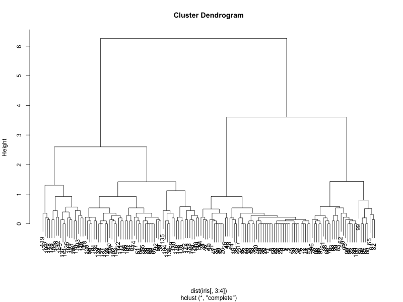
We can see from the figure that the best choices for total number of clusters are either 3 or 4:

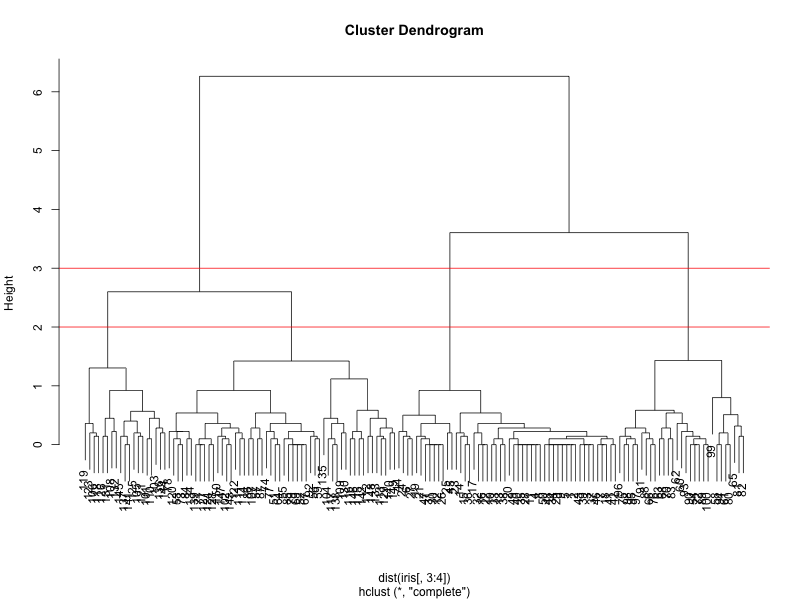
To do this, we can cut off the tree at the desired number of clusters using cutree.

clusterCut <- cutree(clusters, 3)

Now, let us compare it with the original species.

table(clusterCut, iris$Species)
clusterCut setosa versicolor virginica
         1     50          0         0
         2      0         21        50
         3      0         29         0

It looks like the algorithm successfully classified all the flowers of species setosa into cluster 1, and virginica into cluster 2, but had trouble with versicolor. If you look at the original plot showing the different species, you can understand why: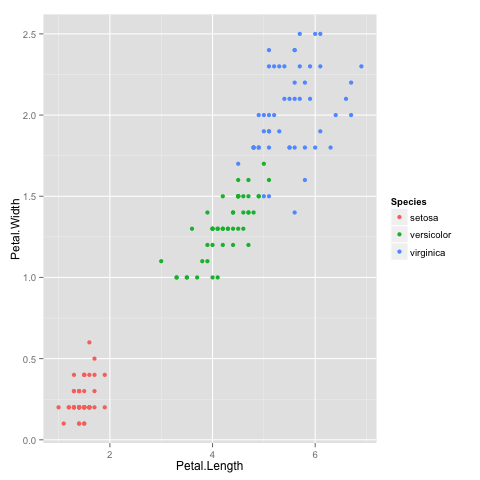

Let us see if we can better by using a different linkage method. This time, we will use the mean linkage method:

clusters <- hclust(dist(iris[, 3:4]), method = 'average')
plot(clusters)

which gives us the following dendrogram:

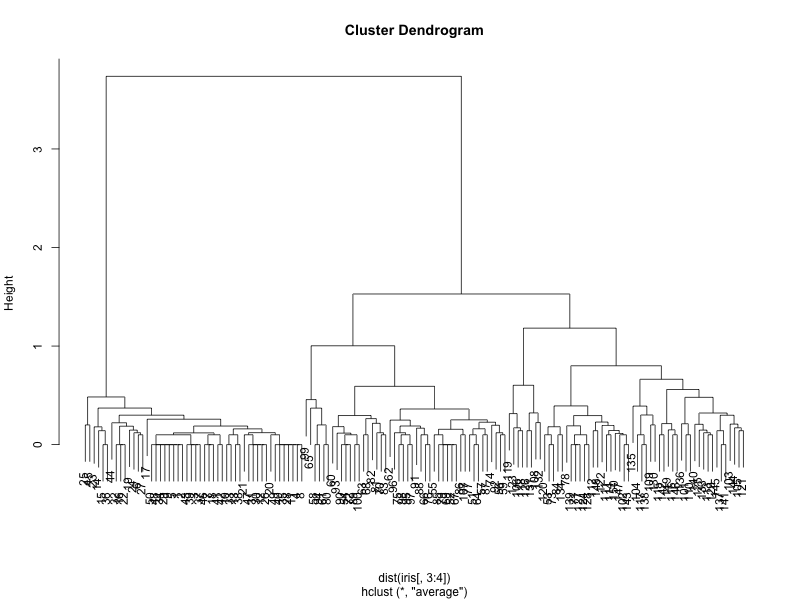
We can see that the two best choices for number of clusters are either 3 or 5. Let us use cutree to bring it down to 3 clusters.

clusterCut <- cutree(clusters, 3)
table(clusterCut, iris$Species)
clusterCut setosa versicolor virginica
         1     50          0         0
         2      0         45         1
         3      0          5        49

We can see that this time, the algorithm did a much better job of clustering the data, only going wrong with 6 of the data points.

We can plot it as follows to compare it with the original data:

ggplot(iris, aes(Petal.Length, Petal.Width, color = iris$Species)) + 
  geom_point(alpha = 0.4, size = 3.5) + geom_point(col = clusterCut) + 
  scale_color_manual(values = c('black', 'red', 'green'))

which gives us the following graph:

All the points where the inner color doesn’t match the outer color are the ones which were clustered incorrectly.

That brings us to the end of this article. If you have any questions or feedback, feel free to leave a comment or reach out to me on Twitter.