Neural networks have always been one of the fascinating machine learning models in my opinion, not only because of the fancy backpropagation algorithm but also because of their complexity (think of deep learning with many hidden layers) and structure inspired by the brain.
Neural networks have not always been popular, partly because they were, and still are in some cases, computationally expensive and partly because they did not seem to yield better results when compared with simpler methods such as support vector machines (SVMs). Nevertheless, Neural Networks have, once again, raised attention and become popular.
Update: We published another post about Network analysis at DataScience+ Network analysis of Game of Thrones
In this post, we are going to fit a simple neural network using the neuralnet package and fit a linear model as a comparison.
The dataset
We are going to use the Boston dataset in the MASS package.
The Boston dataset is a collection of data about housing values in the suburbs of Boston. Our goal is to predict the median value of owner-occupied homes (medv) using all the other continuous variables available.
set.seed(500)
library(MASS)
data <- Boston
First we need to check that no datapoint is missing, otherwise we need to fix the dataset.
apply(data,2,function(x) sum(is.na(x)))
crim      zn   indus    chas     nox      rm     age     dis     rad     tax ptratio
   0       0       0       0       0       0       0       0       0       0       0
black   lstat    medv
    0       0       0
There is no missing data, good. We proceed by randomly splitting the data into a train and a test set, then we fit a linear regression model and test it on the test set. Note that I am using the gml() function instead of the lm() this will become useful later when cross validating the linear model.
index <- sample(1:nrow(data),round(0.75*nrow(data)))
train <- data[index,]
test <- data[-index,]
lm.fit <- glm(medv~., data=train)
summary(lm.fit)
pr.lm <- predict(lm.fit,test)
MSE.lm <- sum((pr.lm - test$medv)^2)/nrow(test)
The sample(x,size) function simply outputs a vector of the specified size of randomly selected samples from the vector x. By default the sampling is without replacement: index is essentially a random vector of indeces.
Since we are dealing with a regression problem, we are going to use the mean squared error (MSE) as a measure of how much our predictions are far away from the real data.
Preparing to fit the neural network
Before fitting a neural network, some preparation need to be done. Neural networks are not that easy to train and tune.
As a first step, we are going to address data preprocessing.
It is good practice to normalize your data before training a neural network. I cannot emphasize enough how important this step is: depending on your dataset, avoiding normalization may lead to useless results or to a very difficult training process (most of the times the algorithm will not converge before the number of maximum iterations allowed). You can choose different methods to scale the data (z-normalization, min-max scale, etc…). I chose to use the min-max method and scale the data in the interval [0,1]. Usually scaling in the intervals [0,1] or [-1,1] tends to give better results.
We therefore scale and split the data before moving on:
maxs <- apply(data, 2, max)
mins <- apply(data, 2, min)
scaled <- as.data.frame(scale(data, center = mins, scale = maxs - mins))
train_ <- scaled[index,]
test_ <- scaled[-index,]
Note that scale returns a matrix that needs to be coerced into a data.frame.
Parameters
As far as I know there is no fixed rule as to how many layers and neurons to use although there are several more or less accepted rules of thumb. Usually, if at all necessary, one hidden layer is enough for a vast numbers of applications. As far as the number of neurons is concerned, it should be between the input layer size and the output layer size, usually 2/3 of the input size. At least in my brief experience testing again and again is the best solution since there is no guarantee that any of these rules will fit your model best.
Since this is a toy example, we are going to use 2 hidden layers with this configuration: 13:5:3:1. The input layer has 13 inputs, the two hidden layers have 5 and 3 neurons and the output layer has, of course, a single output since we are doing regression.
Let’s fit the net:
library(neuralnet)
n <- names(train_)
f <- as.formula(paste("medv ~", paste(n[!n %in% "medv"], collapse = " + ")))
nn <- neuralnet(f,data=train_,hidden=c(5,3),linear.output=T)
A couple of notes:
- For some reason the formula
y~.is not accepted in theneuralnet()function. You need to first write the formula and then pass it as an argument in the fitting function. - The
hiddenargument accepts a vector with the number of neurons for each hidden layer, while the argumentlinear.outputis used to specify whether we want to do regressionlinear.output=TRUEor classificationlinear.output=FALSE
The neuralnet package provides a nice tool to plot the model:
plot(nn)
This is the graphical representation of the model with the weights on each connection:
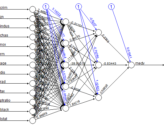
The black lines show the connections between each layer and the weights on each connection while the blue lines show the bias term added in each step. The bias can be thought as the intercept of a linear model.
The net is essentially a black box so we cannot say that much about the fitting, the weights and the model. Suffice to say that the training algorithm has converged and therefore the model is ready to be used.
Predicting medv using the neural network
Now we can try to predict the values for the test set and calculate the MSE. Remember that the net will output a normalized prediction, so we need to scale it back in order to make a meaningful comparison (or just a simple prediction).
pr.nn <- compute(nn,test_[,1:13])
pr.nn_ <- pr.nn$net.result*(max(data$medv)-min(data$medv))+min(data$medv)
test.r <- (test_$medv)*(max(data$medv)-min(data$medv))+min(data$medv)
MSE.nn <- sum((test.r - pr.nn_)^2)/nrow(test_)
we then compare the two MSEs
print(paste(MSE.lm,MSE.nn))
"21.6297593507225 10.1542277747038"
Apparently, the net is doing a better work than the linear model at predicting medv. Once again, be careful because this result depends on the train-test split performed above. Below, after the visual plot, we are going to perform a fast cross validation in order to be more confident about the results.
A first visual approach to the performance of the network and the linear model on the test set is plotted below
par(mfrow=c(1,2))
plot(test$medv,pr.nn_,col='red',main='Real vs predicted NN',pch=18,cex=0.7)
abline(0,1,lwd=2)
legend('bottomright',legend='NN',pch=18,col='red', bty='n')
plot(test$medv,pr.lm,col='blue',main='Real vs predicted lm',pch=18, cex=0.7)
abline(0,1,lwd=2)
legend('bottomright',legend='LM',pch=18,col='blue', bty='n', cex=.95)
The output plot
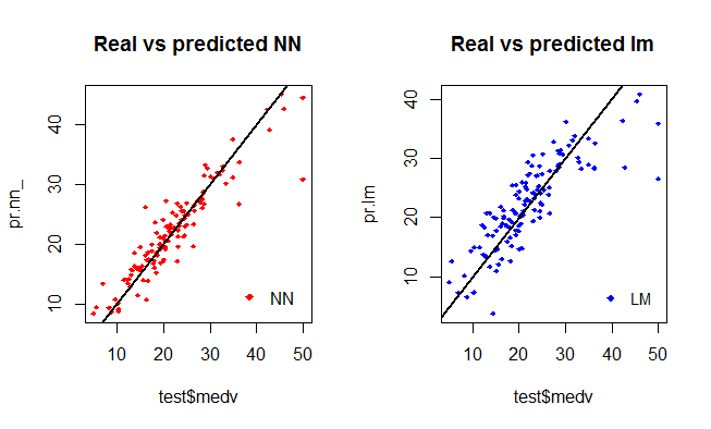
By visually inspecting the plot we can see that the predictions made by the neural network are (in general) more concetrated around the line (a perfect alignment with the line would indicate a MSE of 0 and thus an ideal perfect prediction) than those made by the linear model.
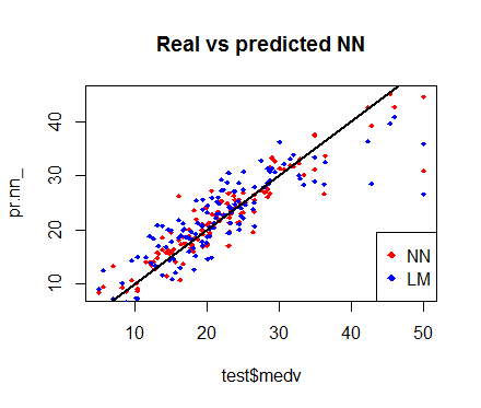
plot(test$medv,pr.nn_,col='red',main='Real vs predicted NN',pch=18,cex=0.7)
points(test$medv,pr.lm,col='blue',pch=18,cex=0.7)
abline(0,1,lwd=2)
legend('bottomright',legend=c('NN','LM'),pch=18,col=c('red','blue'))
A perhaps more useful visual comparison is plotted below:
A (fast) cross validation
Cross validation is another very important step of building predictive models. While there are different kind of cross validation methods, the basic idea is repeating the following process a number of time:
train-test split
- Do the train-test split
- Fit the model to the train set
- Test the model on the test set
- Calculate the prediction error
- Repeat the process K times
Then by calculating the average error we can get a grasp of how the model is doing.
We are going to implement a fast cross validation using a for loop for the neural network and the cv.glm() function in the boot package for the linear model.
As far as I know, there is no built-in function in R to perform cross-validation on this kind of neural network, if you do know such a function, please let me know in the comments. Here is the 10 fold cross-validated MSE for the linear model:
library(boot)
set.seed(200)
lm.fit <- glm(medv~.,data=data)
cv.glm(data,lm.fit,K=10)$delta[1]
23.83560156
Now the net. Note that I am splitting the data in this way: 90% train set and 10% test set in a random way for 10 times. I am also initializing a progress bar using the plyr library because I want to keep an eye on the status of the process since the fitting of the neural network may take a while.
set.seed(450)
cv.error <- NULL
k <- 10
library(plyr)
pbar <- create_progress_bar('text')
pbar$init(k)
for(i in 1:k){
    index <- sample(1:nrow(data),round(0.9*nrow(data)))
    train.cv <- scaled[index,]
    test.cv <- scaled[-index,]
    nn <- neuralnet(f,data=train.cv,hidden=c(5,2),linear.output=T)
    pr.nn <- compute(nn,test.cv[,1:13])
    pr.nn <- pr.nn$net.result*(max(data$medv)-min(data$medv))+min(data$medv)
    test.cv.r <- (test.cv$medv)*(max(data$medv)-min(data$medv))+min(data$medv)
    cv.error[i] <- sum((test.cv.r - pr.nn)^2)/nrow(test.cv)
    pbar$step()
}
After a while, the process is done, we calculate the average MSE and plot the results as a boxplot
mean(cv.error)
cv.error
10.32697995
17.640652805  6.310575067 15.769518577  5.730130820 10.520947119  6.121160840
6.389967211  8.004786424 17.369282494  9.412778105
The code for the box plot:
boxplot(cv.error,xlab='MSE CV',col='cyan',
        border='blue',names='CV error (MSE)',
        main='CV error (MSE) for NN',horizontal=TRUE)
The code above outputs the following boxplot:
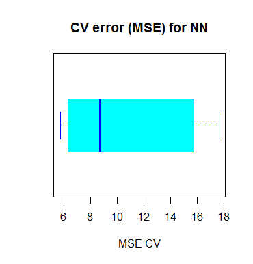
As you can see, the average MSE for the neural network (10.33) is lower than the one of the linear model although there seems to be a certain degree of variation in the MSEs of the cross validation. This may depend on the splitting of the data or the random initialization of the weights in the net. By running the simulation different times with different seeds you can get a more precise point estimate for the average MSE.
A final note on model interpretability
Neural networks resemble black boxes a lot: explaining their outcome is much more difficult than explaining the outcome of simpler model such as a linear model. Therefore, depending on the kind of application you need, you might want to take into account this factor too. Furthermore, as you have seen above, extra care is needed to fit a neural network and small changes can lead to different results.
A gist with the full code for this post can be found here.
Thank you for reading this post, leave a comment below if you have any question.
f <- as.formula(paste("medv ~", paste(n[!n %in% "medv"], collapse = " + "))) can any one explain this formula to me as i stuck with formula on my own data
while applying the formula “f <- as.formula(paste("medv ~", paste(n[!n %in% "medv"], collapse = " + ")))" on my own data i face the following error shown in the image file for your information
How to do the cross validation of Random Forest model.
Am I wrong, or does this use really old optimization algorithms? Is there a NN package with more recent optimizers, like RMSProp?
Thank you, an excellent explanation
it’s amazing~~
Thank you very much Michy! Great article 🙂
Do you know if there is a way to extract the “end-to-end” coefficients of the predictors to the medv variable given the fitted network. So for example:
medv = Coef1*crim+Coef2*Zn+Coef3*Indus+…+TotalBias
Thank you very much Michy. Very useful explanation for begginers.
Next to the NN application I’m searching for a way to figure out which of the input variables is affecting the most the output variable, given the NN fitted model. Is this possible?
Great post! If we decide that NNs are the way to go, then how do you make predictions for new data if we have used the cross validation method. Wouldn’t I have 10 different outcomes since we used K=10?
thank you for this !
hi ,
thanks for sharing such command of R which were very useful for me,
my question is if we time series data then how fit them in this neural net command , as here f <- as.formula(paste("medv ~", paste(n[!n %in% "medv"], collapse = " + ")))
nn <- neuralnet(f,data=train_,hidden=c(5,3),linear.output=T),
but for one variable it doesnt work
kindly suggest here somehow
Great Work, really appreciated. Can you please tell me how to get the predicted values for testing data and make comparison with actual data. Also pls tell can we use neural network for panel data..Best regards
Hi Michy, thanks for the example. I have some questions, is this a good model for time series forecasting? In my study area ( streamflow forecast using precipitation data) is very comom use input data such as image attachments, p is precipitation and q is flow, so p (t-1) is the previous day, which Approach can I use to do this in your example?
Thank you,
Artur https://uploads.disquscdn.com/images/417ebdb24022898ca5f2b5a933dba00ff07e536998046c8b86f7c677bb82c4ed.png
cool, thanks 🙂
Can you please tell me is it k- fold cross validation or repeated k-fold cross validation for the neural network model that you have done here..??
Hello, great post! I was wondering if the same CV procedure for estimating MSE you coded here will work with binomial response data? Thank you!
Thanks nice tuto
if you normalize the data for the linear regression model like NN it will gives you better accuracy than NN
Is there a way to tell the neural network to train only at one train sample at a time? I’ve the feeling that neuralnet is the only method that trains the neural network but once cannot add more train examples to the given network once the method was called. Unless I’m wrong?
Hi Michy, thanks for the code. Quite useful. Couple of questions: 1) what was your reason for using the neuralnet package instead of the more popularly known nnet one that caret supports? Did you find bugs in nnet? I did, that’s why curious.
2) What is your opinion on balancing classes before inputting to the neural network. I have previously used neural nets alot in Matlab where you can actually see the classification boundaries and tell if the net has done a sensible classifcation job, and if I do not do class balance I get rubbish results, especially if in the original dataset there is a significant class imbalance. What do you say, and do you have a code for neural network with balanced classes please? Thanks
Hi Shas, here are my answers:
1) I like the neuralnet package since I find it very user friendly. I have not used nnet very much, so I can’t say anything about it.
2) With a high class imbalance it might be that during training the model is not “giving importance” to the less frequent classes but this should be a common problem for most models, not just for NN.
Personally, I would try to make different experiments, perhaps using weighted samples or weighted random sampling during training, and see in which case you get the best results, as you did.
How to find adjusted R-square/R-square from the linear model of neural net?
Excelent post!!! Thanks!
Nice one.
Cross-validation:
If you already did not know: You can do cross-validation using the caret package as shown below.
library(caret)
model.nnet = train(medv~., data=train,
method=”nnet”,
preProc=c(“center”, “scale”))
print(model.nnet)
I didn’t know that, thanks for sharing!
Hi Michy, a great post and clear explanations. After reading different material on Neural network though I am able to model my data ( though not sure, if correctly!) but in presence of regression models that is so much used in epidemiology, I am not confident whether I should really use neural networks to investigate disease outcomes (causal relationship). Nevertheless, I feel in situations like investigation of biological relationship it should be a valuable method as the biological relationships can be observed in almost any valid data. Could you comment whether neural network can be a valuable method to study biological relationships (e.g. metabolites like cholesterol and disease like Heart diseases?
Interesting question. I work also with medical data and do a lot of regression. However, I never read a paper which applied neural network in their analysis. I am curios how your neural network looks with medical data.
Hi, that is a tough question for me since I have a very limited knowledge of biology. What I can say is that I would prefer other methods over neural networks whenever a causal relationship explanation is required. As far as my knowledge of neural networks goes, they work quite well when you have to tackle a straight classification/regression problem and you don’t really mind about the detailed explanation of why they perfomed well. Having said that, NN are quite good at doing what they do, so there might be some value in using them for pattern recognition to find “study-worthy samples” (especially if you have LOTS of samples) to be further examined using other “less opaque” techniques.
Hey, thank you very much for your explanation! Very useful!
At the moment I’m preparing by data. I’ve scaled metric data on the range 0 to 1 like you, but how would you treat classes? In my dataset there are 3 variable with each 7 classes. If I convert it into binary variables, I will get (3*7=)21 new variables. I’ve tried to run my neural net with it, but it didn’t converge. Could you help me?
Very clearly written and very useful. Thanks.
FYI: I was using dplyr/tidyr + ggplot2 to wrangle & visualize the data in certain ways and I hit a namespace collision for compute() when I ran
pr.nn <- compute(nn, test_[, 1:13])
"Error in UseMethod("compute") : no applicable method for 'compute' applied to an object of class "nn""
I simply had to detach dplyr before running that line successfully.
Thank you for the explanation in detail. Isn’t normalization done only on input variables and not on output variables? Also, would love to see a forecasting post using neuralnet?
Thank you, a very good explanation
Nice ! I read a similar infact exact same chapter in a book … Machine Learning With R by Brett Lantz
Hi Michy.
At a certain row of your paper you plot the results writing:
plot(test$medv,pr.nn_,col=’red’,main=’Real vs Predicted NN’, pch=18,cex=0.7)
You should substitute it with:
plot(test_$medv,pr.nn,col=’red’,main=’Real vs Predicted NN’, pch=18,cex=0.7)
It’s just a little typo. 😉
Andrea
well, i guess you mean plot(test.r,pr.nn_,col=’red’,main=’Real vs Predicted NN’, pch=18,cex=0.7)
It’s just a little typo 😉
Yes, I think that you right parvane, isn’t Michy?
Hi, I like this blog. What do you think the relationship between neural network with multiple layers (e.g., n = 3) and deep learning?
Hi Kong! I appreciate the feedback, thanks! I’m not sure I understand what you are asking, however, it is rare to use more than 1 or 2 layers with this kind of model. One or two layers are usually enough for most applications.
I have not used deep neural networks yet, perhaps in the future I’ll try them out! 🙂
Thank you for your reply. I am new in the neural network, and I think I may start some work with this technique. :)
I liked the walk-through & explanation of this code, but have a question about the normalization step prior to using the neural network. Isn’t normalizing the entire data set “cheating” in this comparison? For this to be more comparable between the linear regression and networking, wouldn’t it be more realistic to normalize the test and training data sets separately.
The lm regression doesn’t get the added information of total range of all data, and is subsequently penalized.
Hi Rich! Thank you for your feedback, I’m glad you liked the post.
The normalization step is almost necessary for the neural network training algorithm to converge nicely (at least in my experience with the neural net package in R) otherwise you could get weird results if any at all.
We assume that the set of predictors X is known before running the model, therefore it is ok to scale the entire set of predictors.
As for y (medv), in the cross validation we use around 90% of the data for the training process, it is reasonable to assume that with that 90% we have an idea of the range of y, so we can approximate by scaling the entire dataset. Of course it could easily happen that the “important” values (max and min of y) are not in the train set, and a deeper validation should dig further into this and try different scenarios and approaches. However, for most of the predictions in this example it should be fine. Using different scales for test and train set is not usually a good idea.
The scaling process doesn’t affect the linear model. You can try to fit the lm and run the cross validation again using a scaled version of the data, however you should get the same results except, of course, different coefficients of the model.
I hope the post doesn’t suggest that neural networks are a better model than linear regression 🙂 Every application is almost unique so we can’t generalize. The linear regression is used as sort of a benchmark to get an idea of how good/bad the net was doing.