
Logistic regression is a method for fitting a regression curve, y = f(x), when y is a categorical variable. The typical use of this model is predicting y given a set of predictors x. The predictors can be continuous, categorical or a mix of both.
The categorical variable y, in general, can assume different values. In the simplest case scenario y is binary meaning that it can assume either the value 1 or 0. A classical example used in machine learning is email classification: given a set of attributes for each email such as a number of words, links, and pictures, the algorithm should decide whether the email is spam (1) or not (0). In this post, we call the model “binomial logistic regression”, since the variable to predict is binary, however, logistic regression can also be used to predict a dependent variable which can assume more than 2 values. In this second case, we call the model “multinomial logistic regression”. A typical example, for instance, would be classifying films between “Entertaining”, “borderline” or “boring”.
Logistic regression implementation in R
R makes it very easy to fit a logistic regression model. The function to be called is glm() and the fitting process is not so different from the one used in linear regression. In this post, I am going to fit a binary logistic regression model and explain each step.
The dataset
We’ll be working on the Titanic dataset. There are different versions of this dataset freely available online, however, I suggest to use the one available at Kaggle since it is almost ready to be used (in order to download it you need to sign up to Kaggle).
The dataset (training) is a collection of data about some of the passengers (889 to be precise), and the goal of the competition is to predict the survival (either 1 if the passenger survived or 0 if they did not) based on some features such as the class of service, the sex, the age etc. As you can see, we are going to use both categorical and continuous variables.
The data cleaning process
When working with a real dataset we need to take into account the fact that some data might be missing or corrupted, therefore we need to prepare the dataset for our analysis. As a first step we load the csv data using the read.csv() function.
Make sure that the parameter na.strings is equal to c("") so that each missing value is coded as a NA. This will help us in the next steps.
training.data.raw <- read.csv('train.csv',header=T,na.strings=c(""))
Now we need to check for missing values and look how many unique values there are for each variable using the sapply() function which applies the function passed as argument to each column of the dataframe.
sapply(training.data.raw,function(x) sum(is.na(x)))
sapply(training.data.raw, function(x) length(unique(x)))
PassengerId    Survived      Pclass        Name         Sex
          0           0           0           0           0
        Age       SibSp       Parch      Ticket        Fare
        177           0           0           0           0
      Cabin    Embarked
        687           2

PassengerId    Survived      Pclass        Name         Sex
        891           2           3         891           2
        Age       SibSp       Parch      Ticket        Fare
         89           7           7         681         248
      Cabin    Embarked
        148           4
A visual take on the missing values might be helpful: the Amelia package has a special plotting function missmap() that will plot your dataset and highlight missing values:
library(Amelia)
missmap(training.data.raw, main = "Missing values vs observed")
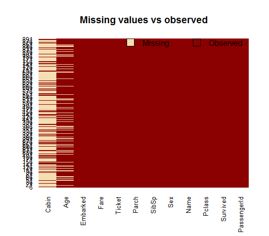
The variable cabin has too many missing values, we will not use it. We will also drop PassengerId since it is only an index and Ticket.
Using the subset() function we subset the original dataset selecting the relevant columns only.
data <- subset(training.data.raw,select=c(2,3,5,6,7,8,10,12))
Taking care of the missing values
Now we need to account for the other missing values. R can easily deal with them when fitting a generalized linear model by setting a parameter inside the fitting function. However, personally, I prefer to replace the NAs “by hand” when is possible. There are different ways to do this, a typical approach is to replace the missing values with the average, the median or the mode of the existing one. I’ll be using the average.
data$Age[is.na(data$Age)] <- mean(data$Age,na.rm=T)
As far as categorical variables are concerned, using the read.table() or read.csv() by default will encode the categorical variables as factors. A factor is how R deals categorical variables.
We can check the encoding using the following lines of code
is.factor(data$Sex)
is.factor(data$Embarked)
TRUE
TRUE
For a better understanding of how R is going to deal with the categorical variables, we can use the contrasts() function. This function will show us how the variables have been dummyfied by R and how to interpret them in a model.
contrasts(data$Sex)
contrasts(data$Embarked)
       male
female    0
male      1

  Q S
C 0 0
Q 1 0
S 0 1
For instance, you can see that in the variable sex, the female will be used as the reference. As for the missing values in Embarked, since there are only two, we will discard those two rows (we could also have replaced the missing values with the mode and keep the data points).
data <- data[!is.na(data$Embarked),]
rownames(data) <- NULL
Before proceeding to the fitting process, let me remind you how important is cleaning and formatting of the data. This preprocessing step often is crucial for obtaining a good fit of the model and better predictive ability.
Model fitting
We split the data into two chunks: training and testing set. The training set will be used to fit our model which we will be testing over the testing set.
train <- data[1:800,]
test <- data[801:889,]
Now, let’s fit the model. Be sure to specify the parameter family=binomial in the glm() function.
model <- glm(Survived ~.,family=binomial(link='logit'),data=train)
By using function summary() we obtain the results of our model:
summary(model)
Call:
glm(formula = Survived ~ ., family = binomial(link = "logit"),
    data = train)

Deviance Residuals:
    Min       1Q   Median       3Q      Max
-2.6064  -0.5954  -0.4254   0.6220   2.4165

Coefficients:
             Estimate Std. Error z value Pr(>|z|)
(Intercept)  5.137627   0.594998   8.635  < 2e-16 ***
Pclass      -1.087156   0.151168  -7.192 6.40e-13 ***
Sexmale     -2.756819   0.212026 -13.002  < 2e-16 ***
Age         -0.037267   0.008195  -4.547 5.43e-06 ***
SibSp       -0.292920   0.114642  -2.555   0.0106 *
Parch       -0.116576   0.128127  -0.910   0.3629
Fare         0.001528   0.002353   0.649   0.5160
EmbarkedQ   -0.002656   0.400882  -0.007   0.9947
EmbarkedS   -0.318786   0.252960  -1.260   0.2076
---
Signif. codes:  0 ‘***’ 0.001 ‘**’ 0.01 ‘*’ 0.05 ‘.’ 0.1 ‘ ’ 1

(Dispersion parameter for binomial family taken to be 1)

    Null deviance: 1065.39  on 799  degrees of freedom
Residual deviance:  709.39  on 791  degrees of freedom
AIC: 727.39

Number of Fisher Scoring iterations: 5
Interpreting the results of our logistic regression model
Now we can analyze the fitting and interpret what the model is telling us.
First of all, we can see that SibSp, Fare and Embarked are not statistically significant. As for the statistically significant variables, sex has the lowest p-value suggesting a strong association of the sex of the passenger with the probability of having survived. The negative coefficient for this predictor suggests that all other variables being equal, the male passenger is less likely to have survived. Remember that in the logit model the response variable is log odds: ln(odds) = ln(p/(1-p)) = a*x1 + b*x2 + … + z*xn. Since male is a dummy variable, being male reduces the log odds by 2.75 while a unit increase in age reduces the log odds by 0.037.
Now we can run the anova() function on the model to analyze the table of deviance
anova(model, test="Chisq")

Analysis of Deviance Table
Model: binomial, link: logit
Response: Survived
Terms added sequentially (first to last)

         Df Deviance Resid. Df Resid. Dev  Pr(>Chi)
NULL                       799    1065.39
Pclass    1   83.607       798     981.79 < 2.2e-16 ***
Sex       1  240.014       797     741.77 < 2.2e-16 ***
Age       1   17.495       796     724.28 2.881e-05 ***
SibSp     1   10.842       795     713.43  0.000992 ***
Parch     1    0.863       794     712.57  0.352873
Fare      1    0.994       793     711.58  0.318717
Embarked  2    2.187       791     709.39  0.334990
---
Signif. codes:  0 ‘***’ 0.001 ‘**’ 0.01 ‘*’ 0.05 ‘.’ 0.1 ‘ ’ 1
The difference between the null deviance and the residual deviance shows how our model is doing against the null model (a model with only the intercept). The wider this gap, the better. Analyzing the table we can see the drop in deviance when adding each variable one at a time. Again, adding Pclass, Sex and Age significantly reduces the residual deviance. The other variables seem to improve the model less even though SibSp has a low p-value. A large p-value here indicates that the model without the variable explains more or less the same amount of variation. Ultimately what you would like to see is a significant drop in deviance and the AIC.
While no exact equivalent to the R2 of linear regression exists, the McFadden R2 index can be used to assess the model fit.
library(pscl)
pR2(model)

         llh      llhNull           G2     McFadden         r2ML         r2CU
-354.6950111 -532.6961008  356.0021794    0.3341513    0.3591775    0.4880244
Assessing the predictive ability of the model
In the steps above, we briefly evaluated the fitting of the model, now we would like to see how the model is doing when predicting y on a new set of data. By setting the parameter type='response', R will output probabilities in the form of P(y=1|X). Our decision boundary will be 0.5. If P(y=1|X) > 0.5 then y = 1 otherwise y=0. Note that for some applications different decision boundaries could be a better option.
fitted.results <- predict(model,newdata=subset(test,select=c(2,3,4,5,6,7,8)),type='response')
fitted.results <- ifelse(fitted.results > 0.5,1,0)
misClasificError <- mean(fitted.results != test$Survived)
print(paste('Accuracy',1-misClasificError))
"Accuracy 0.842696629213483"
The 0.84 accuracy on the test set is quite a good result. However, keep in mind that this result is somewhat dependent on the manual split of the data that I made earlier, therefore if you wish for a more precise score, you would be better off running some kind of cross validation such as k-fold cross validation.
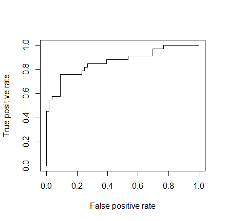
As a last step, we are going to plot the ROC curve and calculate the AUC (area under the curve) which are typical performance measurements for a binary classifier.
The ROC is a curve generated by plotting the true positive rate (TPR) against the false positive rate (FPR) at various threshold settings while the AUC is the area under the ROC curve. As a rule of thumb, a model with good predictive ability should have an AUC closer to 1 (1 is ideal) than to 0.5.
library(ROCR)
p <- predict(model, newdata=subset(test,select=c(2,3,4,5,6,7,8)), type="response")
pr <- prediction(p, test$Survived)
prf <- performance(pr, measure = "tpr", x.measure = "fpr")
plot(prf)

auc <- performance(pr, measure = "auc")
auc <- [email protected][[1]]
auc
0.8647186
And here is the ROC plot:
I hope this post will be useful. A gist with the full code for this example can be found here.
Thank you for reading this post, leave a comment below if you have any question.

I think there is an error: “For instance, you can see that in the variable sex, the female will be used as the reference.” I think “Male” with dummy value = 1 is the reference.
“the female will be used as the reference.” Does this mean that positive estimates represent positive correlation with female and not male?
Well done… But I found it interesting that you’d use the missmap() from Amelia then go on to use the mean for the missing data. Amelia is, after all, a package built for multivariate imputation. I had a chance to use it about a year ago and was very pleased with it. But the ins and outs of Amelia is probably a blog for another day.
It’s perfect content! But, I want to know working about glm, and how can I building a classification model in r without glm function
Please, answer me!
It’s perfect content! But, I want to know working about glm, and how can I building a classification model in r without glm function
Please, answer me!
Great man ,, this is good explanation of Logistic Regression
This is my first step in R, thanks so much!
Hello, thank you for the article, I wanted to implement Logistic Regression using R. But I need help in understanding the interpretation of the results. The result talk about deviance residuals, Estimate, std error, z value, anova, etc. My statistics is not that advanced, please help me in understanding all these terms and their interpretation in Logistic regression.
Thank you!
Thank you for your post. I learned a lot
Firstly, Thanks for this Tutorial The Explanation is very good.
Currently I am working on an Academic Project based on Binomial logistic Regression. Where the response variable is of Binary nature and all the independent variables are of quantitative nature, When i tried visualizing data set i found out that there are so much outliers in the data. So, Should I remove( or replace with central value) ?
Another Problem is that the Correlation Matrix and ggcorrplot is Suggesting Strong Correlation Between some of the independent variables, i.e, Presence of Multicolinearity between variables. In this case how should I Proceed ?
First of all, let me say that I am not an expert. I am currently earning a Master’s degree in Finance, and Business Analytics.
As for the question of outliers, the first thing you should do is go back to your investigation, and try to discover why there are so many outliers. Make sure your data is accurate.
If the data is accurate, then it might be a good idea to eliminate outliers beyond an acceptable threshold as they will skew your data. A standard I often use is 2.5 standard deviations from the mean.
As for Multicolinearity, it usually best to make your model as parsimonious as possible. I would look at running different test models while choosing different independent variables to remove. I would run these through the “glm” and seek the lowest AIC possible. Once I had found the model with the lowest AIC, I would run that model on the test portion of my data. If the model preforms well on the test data, then you have created a model that is generalizable, and not over fit. If you get significantly different AIC score from the train to test portions you have over fit, and need to back and change up your use of independent variables.
I hope this helps!
Excellent post! Many thanks, much appreciatted.
Thanks very much for the step by step explanation. My problem is I tried plotting the logistic curve using ggplot but instead am getting a straight line. Any advice?
I suppose there is a mistake in evaluating the significance of SibSp in the following sentence: “First of all, we can see that SibSp, Fare and Embarked are not statistically significant”. It looks that “Parch” is not significant, SibSp looks significant, is this correct?
I suppose there is a mistake in evaluating the significance of SibSp in the following sentence: “First of all, we can see that SibSp, Fare and Embarked are not statistically significant”. It looks that “Parch” is not significant, SibSp looks significant, is this correct?
A short video tutorial on Logistic Regression for beginners:
https://quickkt.com/tutorials/artificial-intelligence/machine-learning/logistic-regression-theory/
hello pal,
if we import the dataset from a function read.csv(), then by default the categorical variable(s) is(are) converted in factor? or we need to convert it using as.factor() function.
Thanks for your time, very usefull!
Excelente! Muito obrigado!
Excelente article. I have a question… Why in the summary of the model, appear EmbarkedQ and EmbarkedS and not only Embarked? Thanks
What can I do if instead of having the data set I have a contingency table? Should I have to transform it into a data set? Do you have a tutorial for logistic regression with contingency tables?
Hi,
Nice article.
I think I do something wrong because when you calculate the fitted.values on a subset of the test set there are some variable not found.
Maybe it is because the model needs to be recalculated only for the significant variables and then you can calculate the fitted values on a subset of the test set. What do you think?
Anyway it’s not clear how you improve the model. How would you pass from a bad model to one that is good? I would like to find a sort of iterative function that arrives after a certain number of iterations to the best model. I recognise this is difficult, but at least the function could change each time randomly the test set and training set using the sample function, and at each iteration stores some kpi (accuracy, McFadden R^2, significant variables) so that at the end a rank of most significative variables found by accuracy can be given and you can arrive to a sort of general model.
What do you think?
It’s a very good article. Congratulation. I have some question. So you talked about k-fold cross validation. How can we implement this in R in order to improve our model? Namely if we randomly select the rows for the training and test set, then we run the model, we compute the accuracy, and we do as many iterations we want. How can we improve the model from one iteration to the next in order to have a substantially robust model?
Thanks a lot! Regarding ROC to fit models, it is said that Cross validation may be better. Is there a reason for this? What are the weaknesses of ROC vs CV?
I am a newbie to R. Everytime I use model <- glm(formula = Survived ~ .,family=binomial(link='logit'),data=train)
I get an error saying : Error in `contrasts<-`(`*tmp*`, value = contr.funs[1 + isOF[nn]]) :
contrasts can be applied only to factors with 2 or more levels
Could I know where I went wrong and how to correct it?! Thank You!
When my dataset has more than 70% with values equal to ‘0’.. what can i do?
Superb Explanation! Precise description. Thanks a lot! I’m now trying it myself. Will get back in case any queries. 😉
Good post. One thing though, I feel the use of mean substitution for missing values should come with a serious caveat. Now I’m not sure how serious this issue is in logistic, but in linear regression, mean substitution reduces your variance estimate, and can cause that predictor variable to appear significant in a model erroneously. Probably not as big a deal when used on covariates like age.
Thanks for this!!!!
You may be interested to know, but a paperback book is out called Hilbe, Joseph M (2015), “Practical Guide to Logistic Regression” (Chapman & Hall/CRC) that provides detailed modeling guidelines for logistic regression using R. All of the model diagnostics are included as well as complete R code for modeling grouped logistic models, models for unbalanced and perfect prediction, edxact logistic regression, modeling table tata, beta binomial regression for overdispersed grouped logistic models, and complete R and JAGS code for Bayesian logistic models. It’s only about $35 on Amazon. The CRAN package, LOGIT, provides data and a number of specialized R functions for making modeling and presentation easier.
Unsure if you’re still checking up on this (well done) blog, but is there a way to graph the curve by Sensitivity and 1-Specificity? Or are they just tags that can be equally shown by TPR vs FPR?
First, I wanted to congratulate you.
I’ve read several articles, but I haven’t found exactly what I wanted.
I really like your writing, and I wanted to ask if you have any to speak of Interpreting the results of our logistic regression model but with mixed data in R.
I need much of a logistical data example but with mixed data, but with the interpretation of the results, i.e. how to analyze the odds in this case having random part.
In advance I thank you and I apologize for the inconvenience.
God Bless
hello maybe someone can help. I have a couple data sets that i am doing the same thing as this example. in set 1 i get good values and about 4 of 21 variables are sig. and i am able to do a ANOVA. But in my second data set, the test set, i get 1s and .99s (i ran the same analysis on the test set) does that mean that 1 or more of my variables is completely explaining my outcome? that really would not be possible heres what the out put looks like. any advice??? also, i am unable to apply the predictive analysis as in this example to the test set i get errors. im knew to predictive analysis and rstudio in general. thanks
Deviance Residuals:
Min 1Q Median 3Q Max
-1.17741 0.00000 0.00000 0.00001 1.17741
Coefficients:
Estimate Std. Error z value Pr(>|z|)
(Intercept) 2.361e+02 8.046e+05 0.000 1.000
CCNH 3.126e-01 7.269e+02 0.000 1.000
CDK7 -4.434e-01 7.192e+02 -0.001 1.000
DDB1 -4.727e-01 9.034e+02 -0.001 1.000
DDB2 -1.591e+00 1.061e+03 -0.001 0.999
ERCC1 -2.153e-01 5.596e+02 0.000 1.000
ERCC2 6.091e-01 3.247e+03 0.000 1.000
ERCC3 -1.480e+00 2.653e+03 -0.001 1.000
ERCC4 -6.005e+00 1.451e+04 0.000 1.000
ERCC5 3.388e+00 5.403e+03 0.001 0.999
ERCC6 1.152e+00 8.831e+02 0.001 0.999
ERCC8 -5.120e+00 5.698e+03 -0.001 0.999
GTF2H2 1.077e-01 1.918e+03 0.000 1.000
GTF2H3 -6.086e-02 1.996e+02 0.000 1.000
GTF2H4 5.501e-01 1.547e+03 0.000 1.000
RAD23B -1.431e-01 6.344e+02 0.000 1.000
RPA1 6.691e-01 7.038e+02 0.001 0.999
RPA2 1.706e-01 6.174e+02 0.000 1.000
RPA3 6.547e-02 5.579e+02 0.000 1.000
XPA 5.885e-01 8.568e+02 0.001 0.999
XPC 5.662e-02 2.667e+03 0.000 1.000
(Dispersion parameter for binomial family taken to be 1)
Null deviance: 43.6447 on 41 degrees of freedom
Residual deviance: 2.7726 on 21 degrees of freedom
AIC: 44.773
Number of Fisher Scoring iterations: 24
Very interesting and useful post. I will look for your future work. It would have been nicer in some places if you had explained the meaning of some (parts) of the codes that you used, espectially in part “Assessing the predictive ability of the model”. Since you sometimes used multicodes but without explaination, so it was hard to get what their role were. Anyway, I am really enjoyed reading this post. Thanks.
Thanks for the nice work. I really enjoyed reading this whole post. Just have a couple questions. it seems to me that you just tested the separate effect of each predictor like age, sex… on survival probability. However what if some of the factors influence each other and have interactive effect on survival. If I am understand correctly, from this test we can not solve that problem. I am learning this method and also struggle with this isse. It would be nice if you could suggest what should be done to check issue out. Thanks.
Thanks for sharing this.
I tried to execute script but got error for script mentioned in “Assessing the predictive ability of the model”
Below error I am getting
Error in eval(expr, envir, enclos) : object ‘SE.Experities’ not found
Can anyone help me on this
Hi, thanks a lot for this post! i’m new to logistic regression and my question is what’s the difference between logistic regression and classification model in r, since the same example of titanic is used for some people on Kaggle to predict the survival by classification model using rpart in r.
Fantastic walk through of the entire process while building the model. very simple to understand and easy to interpret and follow.
Just couple of questions though:
1) we did not check the C statistics concordant and discordant and other significant parameters such as Somer’s D or gamma value.i use SAS hence i check all these statistics to check strength and direction with the significance of the overall model.
2) as i am pretty new to this domain, hence just wanted to understand why we used type= ‘response’ in accessing the predictive power of the model
Thanks again for putting it out for all of us.
Regards, Shivi
Hi Shivi, thank you for your comment. Indeed, C-statistic is an important statistical test to evaluate the improvement of model discrimination. The c statistic is generally used when you evaluate the new predictor in the model.
Thanks Klodian.
Also if could help with why we used type = response in assessing the predictive power of the model.
Hi Shivi, type = response is new for me as well.
AUC == C == (D+1)/2 for a logistic regression model.
For Goodman-Kruskal gamma and number of other GLM stats at easy access, you might try the lrm method from the rms package in place of glm.
type= ‘response’ simply applies the logistic transform to predicted logodds scores, so the predictions are on the scale of probability.
Thanks for the post. I am new to predictive analytics, I found this post very useful. I want to know just one more thing. if I want to predict failure of a machine for a new month( in this case I wont have the machine ‘fail’ or ‘not fail’ information at the beginning of the month) how can I predict using the predict function?
Actually we should be aware that there is not prediction but an associations (depends on interpretation) between exposure and outcome. If you have information on time when the failure happen then you can do survival analysis (cox regression). For logistic regression the outcome should be yes and no (0, 1). However, there is possible to make an ordinal logistic regression.
Hope I answered your question accordingly.
Thanks for your reply Klodian. I am yet to look into survival analysis. Suppose I have 10 machines with categorical predictors like machine type,location etc. and I want to predict if the machine is going to fail in the next 1 week(fail-1 not fail-0), in this case I want to predict my y as 1 or 0. will I be able to do it with logistic regression?
Suppose my train data is from 1st Jan- 31st July and my test data if from 1st Aug to 31st Aug. From the above mentioned steps, I can fit the data and build a model. now I want to predict, in the first week of Sept how many machines are going to fail? Any thoughts on this if this is possible in logistic regression?
I think logistic regression is the way to go. About survival it works if the failure the machine is not in same time for all machines.
Thanks Klodian!
Thanks for the post. Would it be possible to do a post for when y is a continuous variable and the predictors are a mix of both continuous and categorical variables?
Thanks!
Excellent explanation for a beginner
Hi Michy – this post looks a bit old now, but very helpful, thanks! In your exercise you go through a binomial modelling. Could you give me a one paragraph description regarding what you would do differently if, for example, you wanted to predict the age of a passenger, or fare? I understand that this would be much less accurate, but I would like to understand the process. Could I start by switching the glm function from family=binomial() to something else?
Hello Traveler! Glad to know it’s been useful!
Short answer: to predict a continuous variable you should use linear regression (or another regression model).
Long answer: In the article I tackled a classification problem because y is categorical: in the example y is coded as either 0 or 1 (note that this can be generalized to variables with more than 2 categorical output) however you should not think of y as taking purely numerical values such as 0 or 1 but rather taking a value which is binary such as “blue” or “red”. Then you can code the binary variable as either 0 or 1 and fit a curve using logistic regression, that despite its name, is a powerful classifier (cit. scikit-learn website! 🙂 ).
If you had to predict a continuous variable such as age, then you’d be tackling a regression problem and logistic regression would not be the way to go: you are right, you would get bad results (if any at all). The same applies to linear regression, if you use linear regression to predict a categorical variable such as our y, you may get bad results, such as probabilities that are greater than 1 for some values of the predictor x!
Yes, if you do not set family=binomial(), glm would simply do linear regression (as lm()) and you could easily try to predict your continuous y.
For a better understanding of both the models, I suggest to look at the premises of each of the two models and the problems they were built to solve (you can google both).
I hope I answered your question.
Thank you for really useful post! You wrote: “Note that for some applications different thresholds could be a better option”. Does the threshold depend on the percentage of “success” in the original data set?
Hi Natalja! Thanks for the feedback! 🙂
My bad, I wrote “threshold” where I should have written “decision boundary”! I now corrected it, thanks for pointing that out. The decision boundary is a property, not of the training set, but of the model and of the parameters of the model. That is, the training set is used to fit the parameters that define the decision boundary. Different models fit different decision boundaries.
For a better theoretical explanation, I suggest you to check out the machine learning course by Andrew Ng at Coursera in the “logistic regression” section.
Thanks for this very comprehensive (and comprehensible) article. I particularly appreciate the pains you took to explain the data cleaning processes you employ. I really learnt a lot from it!
Hi BroVic! Thanks for the feedback I appreciate it!
Hi there, first thanks for this clear tutorial. I was just wondering how replacing missing values by average value is a good idea?
Hi Cedric, thank you for the comment. I’m glad you find the tutorial clear.
That’s a good question and a tough one at the same time! 🙂
In general during the fitting stage, what you’d like to do is to keep more data as possible, if there are any NAs in the data, the glm() function, depending on the parameters you set, will stop or drop the missing datapoints. Age is missing 20% of the values so removing 20% of the training set would be a big hit. Replacing the NAs with the mean is a “quick fix” and maintains the mean for age at the same value altough it is a very rough approach. It’s most likely not the best idea, if you were wondering that, you are right. When tuning the model, you may want to try different strategies and see what gets you the best results. For instance, you could do further analysis on the Age variable, see how it relates to the other features (say Pclass, Sex, the title, the Fare etc..) and make more “informed” substitutions e.g. substitute the missing age based on the average age for a certain subgroup of passenger that have the same characteristics etc.. There are many different ways to deal with missing values, perhaps in the future we’ll make a post on that! I hope I answered your question!