Missing data can be a not so trivial problem when analysing a dataset and accounting for it is usually not so straightforward either. If the amount of missing data is very small relatively to the size of the dataset, then leaving out the few samples with missing features may be the best strategy in order not to bias the analysis, however leaving out available datapoints deprives the data of some amount of information and depending on the situation you face, you may want to look for other fixes before wiping out potentially useful datapoints from your dataset.
Update
A simplified approach to impute missing data with MICE package can be found there: Handling missing data with MICE package; a simple approach.
While some quick fixes such as mean-substitution may be fine in some cases, such simple approaches usually introduce bias into the data, for instance, applying mean substitution leaves the mean unchanged (which is desirable) but decreases variance, which may be undesirable.
The mice package in R, helps you imputing missing values with plausible data values. These plausible values are drawn from a distribution specifically designed for each missing datapoint.
In this post we are going to impute missing values using a the airquality dataset (available in R).
For the purpose of the article I am going to remove some datapoints from the dataset.
data <- airquality
data[4:10,3] <- rep(NA,7)
data[1:5,4] <- NA
As far as categorical variables are concerned, replacing categorical variables is usually not advisable. Some common practice include replacing missing categorical variables with the mode of the observed ones, however, it is questionable whether it is a good choice. Even though in this case no datapoints are missing from the categorical variables, we remove them from our dataset (we can add them back later if needed) and take a look at the data using summary().
data <- data[-c(5,6)]
summary(data)

     Ozone           Solar.R           Wind             Temp
 Min.   :  1.00   Min.   :  7.0   Min.   : 1.700   Min.   :57.00
 1st Qu.: 18.00   1st Qu.:115.8   1st Qu.: 7.400   1st Qu.:73.00
 Median : 31.50   Median :205.0   Median : 9.700   Median :79.00
 Mean   : 42.13   Mean   :185.9   Mean   : 9.806   Mean   :78.28
 3rd Qu.: 63.25   3rd Qu.:258.8   3rd Qu.:11.500   3rd Qu.:85.00
 Max.   :168.00   Max.   :334.0   Max.   :20.700   Max.   :97.00
 NA's   :37       NA's   :7       NA's   :7        NA's   :5
Apparently Ozone is the variable with the most missing datapoints. Below we are going to dig deeper into the missing data patterns.
Quick classification of missing data
There are two types of missing data:
- MCAR: missing completely at random. This is the desirable scenario in case of missing data.
- MNAR: missing not at random. Missing not at random data is a more serious issue and in this case it might be wise to check the data gathering process further and try to understand why the information is missing. For instance, if most of the people in a survey did not answer a certain question, why did they do that? Was the question unclear?
Assuming data is MCAR, too much missing data can be a problem too. Usually a safe maximum threshold is 5% of the total for large datasets. If missing data for a certain feature or sample is more than 5% then you probably should leave that feature or sample out. We therefore check for features (columns) and samples (rows) where more than 5% of the data is missing using a simple function
pMiss <- function(x){sum(is.na(x))/length(x)*100}
apply(data,2,pMiss)
apply(data,1,pMiss)

    Ozone   Solar.R      Wind      Temp
24.183007  4.575163  4.575163  3.267974

  [1]  25  25  25  50 100  50  25  25  25  50  25   0   0   0   0   0   0   0   0   0   0
 [22]   0   0   0  25  25  50   0   0   0   0  25  25  25  25  25  25   0  25   0   0  25
 [43]  25   0  25  25   0   0   0   0   0  25  25  25  25  25  25  25  25  25  25   0   0
 [64]   0  25   0   0   0   0   0   0  25   0   0  25   0   0   0   0   0   0   0  25  25
 [85]   0   0   0   0   0   0   0   0   0   0   0  25  25  25   0   0   0  25  25   0   0
[106]   0  25   0   0   0   0   0   0   0  25   0   0   0  25   0   0   0   0   0   0   0
[127]   0   0   0   0   0   0   0   0   0   0   0   0   0   0   0   0   0   0   0   0   0
[148]   0   0  25   0   0   0
We see that Ozone is missing almost 25% of the datapoints, therefore we might consider either dropping it from the analysis or gather more measurements. The other variables are below the 5% threshold so we can keep them. As far as the samples are concerned, missing just one feature leads to a 25% missing data per sample. Samples that are missing 2 or more features (>50%), should be dropped if possible.
Using mice for looking at missing data pattern
The mice package provides a nice function md.pattern() to get a better understanding of the pattern of missing data
library(mice)
md.pattern(data)

    Temp Solar.R Wind Ozone
104    1       1    1     1  0
 34    1       1    1     0  1
  4    1       0    1     1  1
  3    1       1    0     1  1
  3    0       1    1     1  1
  1    1       0    1     0  2
  1    1       1    0     0  2
  1    1       0    0     1  2
  1    0       1    0     1  2
  1    0       0    0     0  4
       5       7    7    37 56
The output tells us that 104 samples are complete, 34 samples miss only the Ozone measurement, 4 samples miss only the Solar.R value and so on.
A perhaps more helpful visual representation can be obtained using the VIM package as follows
library(VIM)
aggr_plot <- aggr(data, col=c('navyblue','red'), numbers=TRUE, sortVars=TRUE, labels=names(data), cex.axis=.7, gap=3, ylab=c("Histogram of missing data","Pattern"))
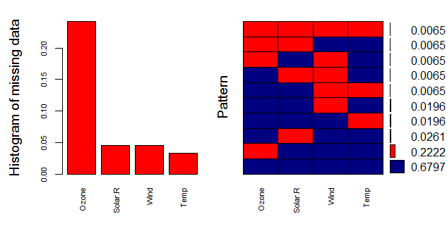
The plot helps us understanding that almost 70% of the samples are not missing any information, 22% are missing the Ozone value, and the remaining ones show other missing patterns. Through this approach the situation looks a bit clearer in my opinion.
Another (hopefully) helpful visual approach is a special box plot
marginplot(data[c(1,2)])

Obviously here we are constrained at plotting 2 variables at a time only, but nevertheless we can gather some interesting insights.
The red box plot on the left shows the distribution of Solar.R with Ozone missing while the blue box plot shows the distribution of the remaining datapoints. Likewhise for the Ozone box plots at the bottom of the graph.
If our assumption of MCAR data is correct, then we expect the red and blue box plots to be very similar.
Imputing the missing data
The mice() function takes care of the imputing process
tempData <- mice(data,m=5,maxit=50,meth='pmm',seed=500)
summary(tempData)

Multiply imputed data set
Call:
mice(data = data, m = 5, method = "pmm", maxit = 50, seed = 500)
Number of multiple imputations:  5
Missing cells per column:
  Ozone Solar.R    Wind    Temp
     37       7       7       5
Imputation methods:
  Ozone Solar.R    Wind    Temp
  "pmm"   "pmm"   "pmm"   "pmm"
VisitSequence:
  Ozone Solar.R    Wind    Temp
      1       2       3       4
PredictorMatrix:
        Ozone Solar.R Wind Temp
Ozone       0       1    1    1
Solar.R     1       0    1    1
Wind        1       1    0    1
Temp        1       1    1    0
Random generator seed value:  500
A couple of notes on the parameters:
-
m=5refers to the number of imputed datasets. Five is the default value. -
meth='pmm'refers to the imputation method. In this case we are using predictive mean matching as imputation method. Other imputation methods can be used, typemethods(mice)for a list of the available imputation methods.
If you would like to check the imputed data, for instance for the variable Ozone, you need to enter the following line of code
tempData$imp$Ozone

      1  2   3   4   5
5    13 20  28  12   9
10    7 16  28  14  20
25    8 14  14   1   8
26    9 19  32   8  37
...
The output shows the imputed data for each observation (first column left) within each imputed dataset (first row at the top).
If you need to check the imputation method used for each variable, mice makes it very easy to do
tempData$meth

  Ozone Solar.R    Wind    Temp
  "pmm"   "pmm"   "pmm"   "pmm"
Now we can get back the completed dataset using the complete() function. It is almost plain English:
completedData <- complete(tempData,1)
The missing values have been replaced with the imputed values in the first of the five datasets. If you wish to use another one, just change the second parameter in the complete() function.
Inspecting the distribution of original and imputed data
Let’s compare the distributions of original and imputed data using a some useful plots.
First of all we can use a scatterplot and plot Ozone against all the other variables
xyplot(tempData,Ozone ~ Wind+Temp+Solar.R,pch=18,cex=1)
Here it is
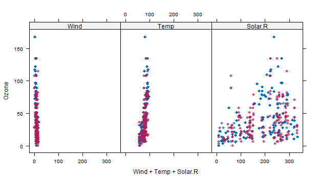
What we would like to see is that the shape of the magenta points (imputed) matches the shape of the blue ones (observed). The matching shape tells us that the imputed values are indeed “plausible values”.
Another helpful plot is the density plot:
densityplot(tempData)
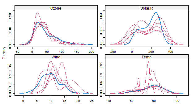
The density of the imputed data for each imputed dataset is showed in magenta while the density of the observed data is showed in blue. Again, under our previous assumptions we expect the distributions to be similar.
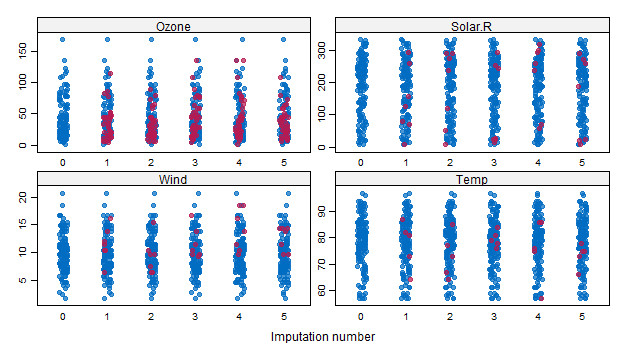
Another useful visual take on the distributions can be obtained using the stripplot() function that shows the distributions of the variables as individual points
stripplot(tempData, pch = 20, cex = 1.2)
Pooling
Suppose that the next step in our analysis is to fit a linear model to the data. You may ask what imputed dataset to choose. The mice package makes it again very easy to fit a a model to each of the imputed dataset and then pool the results together
modelFit1 <- with(tempData,lm(Temp~ Ozone+Solar.R+Wind))
summary(pool(modelFit1))

                     est         se         t       df     Pr(>|t|)
(Intercept) 72.812078768 2.95380500 24.650266 84.18464 0.000000e+00
Ozone        0.163094287 0.02607674  6.254397 57.78569 5.236295e-08
Solar.R      0.009679676 0.00789576  1.225933 37.48960 2.278691e-01
Wind        -0.352582008 0.21639828 -1.629320 92.89136 1.066321e-01
                   lo 95       hi 95 nmis       fmi    lambda
(Intercept) 66.938301817 78.68585572   NA 0.1477818 0.1277731
Ozone        0.110891894  0.21529668   37 0.2155848 0.1888975
Solar.R     -0.006311604  0.02567095    7 0.3004189 0.2640672
Wind        -0.782312735  0.07714872    0 0.1300747 0.1115442
The variable modelFit1 containts the results of the fitting performed over the imputed datasets, while the pool() function pools them all together. Apparently, only the Ozone variable is statistically significant.
Note that there are other columns aside from those typical of the lm() model: fmi contains the fraction of missing information while lambda is the proportion of total variance that is attributable to the missing data. For more information I suggest to check out the paper cited at the bottom of the page.
Remember that we initialized the mice function with a specific seed, therefore the results are somewhat dependent on our initial choice. To reduce this effect, we can impute a higher number of dataset, by changing the default m=5 parameter in the mice() function as follows
tempData2 <- mice(data,m=50,seed=245435)
modelFit2 <- with(tempData2,lm(Temp~ Ozone+Solar.R+Wind))
summary(pool(modelFit2))

                     est          se         t       df     Pr(>|t|)
(Intercept) 73.156084276 2.803010282 26.099114 129.3154 0.000000e+00
Ozone        0.166242781 0.024926976  6.669192 118.4408 8.645631e-10
Solar.R      0.009046835 0.007374103  1.226839 114.5471 2.223989e-01
Wind        -0.382700790 0.202976584 -1.885443 136.6735 6.149264e-02
                   lo 95       hi 95 nmis        fmi    lambda
(Intercept) 67.610387851 78.70178070   NA 0.11141367 0.0977762
Ozone        0.116882484  0.21560308   37 0.16290744 0.1488906
Solar.R     -0.005560458  0.02365413    7 0.18096774 0.1667911
Wind        -0.784081566  0.01867999    0 0.07425875 0.0608104
After having taken into account the random seed initialization, we obtain (in this case) more or less the same results as before with only Ozone showing statistical significance.
A gist with the full code for this post can be found here.
Thank you for reading this post, leave a comment below if you have any question.
Note: I learnt this technique in a paper entitled mice: Multivariate Imputation by Chained Equations in R by Stef van Buuren. It is a great paper and I highly recommend to read it if you are interested in multiple imputation!


Hi! Thank you so much for this article – it was really useful. I am confused about one thing though. You use the complete function to merge your old dataset with one of the imputed datasets, but then never end up using it… Are we meant to run our regression analyses using completed datasets or the purely imputed datasets? Because it seems to me that the output of the mice function includes datapoints all of which have been imputed, rather than purely the missing ones. So does it make sense to use the pure output of the mice function to run regression analyses?
Excellent explanation. Thanks in advance…
Hi! This post was extremely helpful. I am trying to pool my datasets together but I keep getting this error. Any tips?
Error in mutate_impl(.data, dots) : Evaluation error: argument “value” is missing, with no default.
Very helpful article on mice. One question though: when I tried xyplot, I got a message from R: Error: could not find function “xyplot”; likewise for densityplot, stripplot. I was not able to work around this. Any suggestions? Thanks!
Very interesting and I have learned a lot from this write up. Thank you.
Hi all, I have used the above to build my own machine learning tool and all that remains is for me to incorporate this into Power BI so that it becomes a complete tool. The lines of code worked well for my NPS (net promoter score) data. All my lines of code (in using MICE for multivariate imputation.)
Hi, thanks for this. Perhaps a silly questions, but how’d you get your
summary()to display the info and headers you have i.e.,est se t df Pr(>|t|) lo 95 hi 95 nmis fmi lambda? Thanks.this is my code for mice and relative error:
“`
newimp<-mice(df1,m=28,seed=1)
system is computationally singular: reciprocal condition number = 2.14226e-16
newimp<-mice(df1,m=28,seed=1,method='cart')
modelFit1 <- with(newimp,lm(iupm_yr2~.,data=newimp))
Error in as.data.frame.default(data) :
cannot coerce class ‘"mids"’ to a data.frame
“`
Hi, thanks for the article, great work. I would like to use the package to impute data from a clinical trial, in which I have two groups (i.e. control =0; intervention=1). I want to impute the missing data separately for each group, using the same imputation model. So, I do not want to use group, as a categorical predictor (0;1) but actually perform separate imputations. Do you know an efficient way to do so? Thank you.
Hello, thank you for this very helpful tutorial.
However, when I run the provided code, I obtain an error after using the complete() function:
<>
I get the same error reported when I perform the imputation using my own data.
Anyone knows what this error means? Does it have something to do with uninstalled packages?
Thank you in advance,
Alba.
Make sure you have installed and loaded the package mice.
install.packages(“mice”)
library(mice)
Awesome article. Very easy to learn and understand.
Just one small problem. The xyplot function is not working.
Thanks
Thank you for writing this article, as it was very helpful. But I do have a question that I’m hoping someone can shed some light on. Instead of using the complete() function to select a specific data set for inputting missing data, is there a method that can be used to pool together the data sets (m=5) in order to generate a data set that provides the best estimated values for those that are missing? Also, it’s unclear as to what the seed value does or is used for. Does a seed need to be specified?
Thanks in advance!!
You can pool the regression coefiecents. I did this some times ago but I do not recall it now which function I used. I suggest to google your question.
Hi Michy,
A much needed post. Thank you!
I’ve done for m= 5 and now how can I chose best out of 5 imputed sets or how to get the avarage of the five sets for more accurate results.
This is a great post! Thank you!
The one thing I can’t get is: if we already imputed the values – why do we need to fit a linear model in addition?
Pretty good post. I am new to misssing data analysis. Now I want to divide dataset into train and test. I use train data to fit a mice model. How can I use this model to impute my test set and predict the Y?
Did you get answer to your question? Even I’m looking for an answer.
Hello Michy
Excellent Post, congrats for it !!!
I need help to evaluate / choose the best imputation from dichotomic data.
ps: I am not going to fit a linear model, I will use the complete data to build a Bayesian Network, so my objective is to run multiple imputation and then for each variable choose the best imputated data.
Let me know if I am wrong:
Using continuous data I can do:
imp <- mice(mydata, m=5, maxit = 50,method = 'pmm', seed = 500)
fit1 <- with(imp, lm(V1~V2+V3))
fit2 <- with(imp, lm(V2~V1+V3))
fit3 <- with(imp, lm(V3~V1+V2))
then doing summary(ftn) I can evaluate Residual standard error, Multiple R-squared and p-value to choose what is the best imputation (low error and higher R2 with significant p).
Using dichotomic data, I can use:
fit4 <- with(imp, glm(V3~V1+V2, famlily=binomial, (link="logit"))
So I tried but did not found Residual standard error, Multiple R-squared and p-value on the results, what I have found is:
Degrees of Freedom: 29 Total (i.e. Null); 27 Residual
Null Deviance: 38.19
Residual Deviance: 18.71 AIC: 24.71
I am new on imputation data and in regressions, so can you help me in how to evaluate the best imputed dataset for each variable?
Tks
Hello ?????
I used it. But what is the result??? I mean what is the replace number? How can I know? In summary(pool(modelFit2))??
Good information!!!
But i have a question.
Can i replace factor data type as using mice package?
In this post, I saw it isn’t advisable.
Hi there,
No matter what I do I keep getting the error “Error in pool(modFit1) : The object must have class ‘mira'” when I try to pool the data. I am able to generate the different values but pooling doesnt happen because of this error. Can you provide any help?
I followed the tutorial closely but am getting the error message nonetheless. Any thoughts as to what the specific problem might be?
Hello Michy! Thanks for this useful article! I am new in imputation techniques and I started using mice(), but I am not sure if my results are correct. In my results I see that the imputed values are actually values that already exist in the observed values of the same attribute. I expected that the imputed values would be totally new values depending on the rest attributes (as specified in the PredictorMatrix).
Do I do something wrong?
dsgn<-quickpred(data, minpuc = 0.01)
temp<-mice(data,m=5, maxit=2,meth="rf", predictorMatrix =dsgn, visitSequence = "monotone", seed=777)
"data" contains only numerical values
I have employed different methods like pmm, mean etc.
Thanks in advance!
Great Klodian! Thank you very much! I hadn’t realized that my data were recognized as factors, so after the transformation to numeric values everything is fine!
Nice post! I have used the mice package as per the above R-script but when I change the sequence of my variables in the dataset, the pooled estimates are quite different.
OriginalMI <- read.csv ("imputationR.csv")
OriginalMI1 <- subset(OriginalMI, select=c(2:23))
ImputeData < mice(OriginalMI1,m=5,maxit=50,meth='pmm',seed=1986)
Did I did something wrong?
I was also trying to use the imputed data set to check the discrimination and calibration index using PredictABEL package but Am not able to pool the results.
Do a single imputation and use that dataset with PredictABEL.
Thank you for your prompt response. I have tried using single imputation but it does not solve the problem as well. I encounter the same problem like my previous MI.
Sec. Ques: Does changing the column sequence of the variable will have an impact in logit output after MI?
Many thanks for your well-thought out posts and prompt responses. The materials were also very helpful for me!
Hi Michy,
I followed your directions, which were great, but my imputation has been running for 8 hours now, and I’m not sure if this is right. My data set only has 3,000 entries, and of them only 60 or so are missing. Does this seem like the right amount of time to you?
Hi, once I use the complete function, I am getting the error:
Error in (function (classes, fdef, mtable) :
unable to find an inherited method for function ‘complete’ for signature ‘”mids”, “numeric”’
Kindly help.
I have a dataset with 20,000 columns and it is taking forever for the data to impute (48 hours), could you please suggest me an efficient way to do this.
MICE code i used :
tempData <- mice(data,m=1,maxit=50,meth='norm',seed=500, printFlag=FALSE)
Great post!
I’m trying to limit the imputation of missing data with mice package in order to not input all the missing data, i.e, to still keep some missing data . Do you know if it’s possible to do it with the mice package?Thank you!!
Thanks. Things like: meth[c(“Age”)]=”” ,could be also useful.
My issue it’s a bit different.
I have “n” rows and “k” variables. Each row represents a village and 3 of the “k” variables that I would like to impute are “total numer of houses”, “first houses” and “second houses”, where Total = First + Second. So first I handle the missing data of the total houses and then I should handle the other ones. I know that before the imputacion the proportion of “informed first houses/ informed total houses” was 85% and 15% for the second houses, so my goal it’s not to input all de NAs of the variables “first houses” and “second houses”, because I would like to keep some NAs in each variable in order to keep the proportion. I didn’t found the option of fixing a limit of imputed NAs in each variable in the package. I hope it was understood. Thanks again!
when i am working out the above code i am facing the below problem
install.packages(“VIM”)
Installing package into ‘C:/Users/venky/Documents/R/win-library/3.3’
(as ‘lib’ is unspecified)
Warning in install.packages :
package ‘VIM’ is not available (for R version 3.3.1)
you have to install the VIM package for plotting..It is as simple as the error
Very interesting post. I am new to Analytics with R, and had a problem in analyzing data with missing examples. I was stuck on imputing with only one data set from the mice function, but I have gotten a key takeaway from this post in that I can now pool together multiple imputed data sets.
> Even though in this case no datapoints are missing from the categorical variables, we remove them from our dataset (we can add them back later if needed) and take a look at the data using summary().
How do I add my categorical variables back? Thanks.
Wouldn’t it make sense to get the average of the “data set” imputations? So in the command “complete(tempData,1)” it seems like we are only getting one imputation value, so why would it matter how many imputations we do? So, later in the code the imputation number is changed to 50 and the seed is higher, which I would think would make a better prediction. But then how do I get the average of those 50 imputations for each variable? Also, I don’t know if I am getting this correct, but are these imputations made based on the other variables in my data set or are the variables thought to be independent? So are the imputations made within just one variable or is it looking at the other variables in the data set to get the information. Sorry for so many questions. I am just trying to figure out what the code is actually doing. I would appreciate any help anyone can give.
Another question is for the md.pattern function, can you then get the average for certain variables given those conditions in that md.pattern table?
This is assuming that the data is missing at random? When you are looking for “plausible” values isn’t that with the expectation that the missing values are going to be similar to observed values? My data (in a survey) is not missing at random and average for the missing scores are probably biased in a negative fashion (which you could probably see if you did some sort of cross-analysis). Thanks.
I’m working with panel data in wide format. The observed years are 1919-2007, and the data set is a 200×891 matrix. That’s 200 countries, a column for the country ID (column 1), and 10 variables. Two of the variables are ordinal and one is dichotomous, so since pmm is appropriate for continuous variables, I need mice to use the logreg and polr methods for the dichotomous and ordinal variables, respectively. How can I get mice to “loop” over using the pattern of appropriate methods, for each year?
When I attempt to call densityplot I receive the following error:
Error: could not find function “densityplot”
I am using a Mac, Mavericks and R studio. Both R and R Studio were upgrade on 12-18-2015.
Try to load the package: library(lattice)
Hi Michy,
Very useful post. How can I return the final data set using the final model from 50 imputation?
Many thanks
Hello Rafik! Thanks!
To get back, say the nth imputed dataset (n < m), you can type:
imputed_n <- complete(tempData,action=n)
If instead you want to recover all the imputed dataset, then type:
imputed_all <- complete(tempData,action='long')
Note that all the dataset will be stacked into a single dataframe.
I hope it answers your question.
Many thanks again Michy.
You exactly answered my question.
All the best.
Great post! I’d like to point out this simple comparison of imputation methods in the presence of categorical data I have published a couple of years ago:
http://siba-ese.unisalento.it/index.php/ejasa/article/view/12336
you can download the full text pdf there.
Mice is among the considered methods.
Again, nice work!
Hi Federico! Thank you for your kind words and for the paper suggestion! I’ve added it to my to-read list
Thanks for this helpful demonstration. One suggestion; the MICE algorithm is a MCMC method (a Gibbs sampler when all conditionals are compatible). It is wise to inspect the trace-lines to assess convergence. This can be simply done in MICE by
plot(TempData2)
Again, thanks for this walkthrough example.
– Gerko
Hi Gerko! Thanks for pointing that out!
The paper suggests to do this too, however, for some reason that command did not work on this example on my pc (I kept getting an incomplete plot) and then I forgot to add this information in the post!
Excellent post! Thank you. It’s clever. (or as we say in the NYC area– clevuh !)
Thanks for your kind comment! I’m very glad you like the post!