Random Forests in R

Ensemble Learning is a type of Supervised Learning Technique in which the basic idea is to generate multiple Models on a training dataset and then simply combining(average) their Output Rules or their Hypothesis \( H_x \) to generate a Strong Model which performs very well and does not overfits and which balances the Bias-Variance Tradeoff too.

The idea is that instead of producing a single complicated and complex Model which might have a high variance which will lead to Overfitting or might be too simple and have a high bias which leads to Underfitting, we will generate lots of Models by training on Training Set and at the end combine them. Such a technique is Random Forest which is a popular Ensembling technique is used to improve the predictive performance of Decision Trees by reducing the variance in the Trees by averaging them. Decision Trees are considered very simple and easily interpretable as well as understandable Modelling techniques, but a major drawback in them is that they have a poor predictive performance and poor Generalization on Test Set. They are also referred to as Weak Learners which are Learners which always perform better than chance and have an error less than 50 %.

Random Forests

Random Forests are similar to a famous Ensemble technique called Bagging but have a different tweak in it. In Random Forests the idea is to decorrelate the several trees which are generated by the different bootstrapped samples from training Data. And then we simply reduce the Variance in the Trees by averaging them.
Averaging the Trees helps us to reduce the variance and also improve the Performance of Decision Trees on Test Set and eventually avoid Overfitting.

The idea is to build lots of Trees in such a way to make the Correlation between the Trees smaller.

Another major difference is that we only consider a Random subset of predictors \( m \) each time we do a split on training examples. Whereas usually in Trees we find all the predictors while doing a split and choose best amongst them. Typically \( m=\sqrt{p} \) where \(p\) are the number of predictors.

Now it seems crazy to throw away lots of predictors, but it makes sense because the effect of doing so is that each tree uses different predictors to split data at various times. This means that 2 trees generated on same training data will have randomly different variables selected at each split, hence this is how the trees will get de-correlated and will be independent of each other. Another great thing about Random Forests and Bagging is that we can keep on adding more and more big bushy trees and that won’t hurt us because at the end we are just going to average them out which will reduce the variance by the factor of the number of Trees \(T\) itself.

So by doing this trick of throwing away Predictors, we have de-correlated the Trees and the resulting average seems a little better.

Implementation in R

loading the required packages

require(randomForest)
require(MASS)#Package which contains the Boston housing dataset
attach(Boston)
set.seed(101)

dim(Boston)
## [1] 506  14

Saperating Training and Test Sets

#training Sample with 300 observations
train=sample(1:nrow(Boston),300)
?Boston  #to search on the dataset

We are going to use variable ′medv′ as the Response variable, which is the Median Housing Value. We will fit 500 Trees.

Fitting the Random Forest

We will use all the Predictors in the dataset.

Boston.rf=randomForest(medv ~ . , data = Boston , subset = train)
Boston.rf
## 
## Call:
##  randomForest(formula = medv ~ ., data = Boston, subset = train) 
##                Type of random forest: regression
##                      Number of trees: 500
## No. of variables tried at each split: 4
## 
##           Mean of squared residuals: 12.62686
##                     % Var explained: 84.74

The above Mean Squared Error and Variance explained are calculated using Out of Bag Error Estimation.In this \(\frac23\) of Training data is used for training and the remaining \( \frac13 \) is used to Validate the Trees. Also, the number of variables randomly selected at each split is 4.

Plotting the Error vs Number of Trees Graph.

plot(Boston.rf)

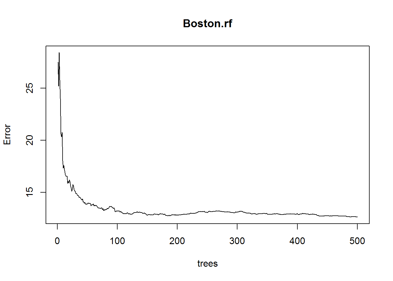
This plot shows the Error and the Number of Trees. We can easily notice that how the Error is dropping as we keep on adding more and more trees and average them.

Now we can compare the Out of Bag Sample Errors and Error on Test set

The above Random Forest model chose Randomly 4 variables to be considered at each split. We could now try all possible 13 predictors which can be found at each split.

oob.err=double(13)
test.err=double(13)

#mtry is no of Variables randomly chosen at each split
for(mtry in 1:13) 
{
  rf=randomForest(medv ~ . , data = Boston , subset = train,mtry=mtry,ntree=400) 
  oob.err[mtry] = rf$mse[400] #Error of all Trees fitted
  
  pred<-predict(rf,Boston[-train,]) #Predictions on Test Set for each Tree
  test.err[mtry]= with(Boston[-train,], mean( (medv - pred)^2)) #Mean Squared Test Error
  
  cat(mtry," ") #printing the output to the console
  
}
## 1  2  3  4  5  6  7  8  9  10  11  12  13

Test Error

test.err
##  [1] 26.06433 17.70018 16.51951 14.94621 14.51686 14.64315 14.60834
##  [8] 15.12250 14.42441 14.53687 14.89362 14.86470 15.09553

Out of Bag Error Estimation

oob.err
##  [1] 19.95114 13.34894 13.27162 12.44081 12.75080 12.96327 13.54794
##  [8] 13.68273 14.16359 14.52294 14.41576 14.69038 14.72979

What happens is that we are growing 400 trees for 13 times i.e for all 13 predictors.

Plotting both Test Error and Out of Bag Error

matplot(1:mtry , cbind(oob.err,test.err), pch=19 , col=c("red","blue"),type="b",ylab="Mean Squared Error",xlab="Number of Predictors Considered at each Split")
legend("topright",legend=c("Out of Bag Error","Test Error"),pch=19, col=c("red","blue"))

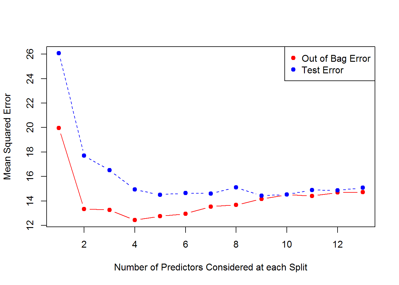
Now what we observe is that the Red line is the Out of Bag Error Estimates and the Blue Line is the Error calculated on Test Set. Both curves are quite smooth and the error estimates are somewhat correlated too. The Error Tends to be minimized at around \( mtry = 4 \).

On the Extreme Right Hand Side of the above plot, we considered all possible 13 predictors at each Split which is only Bagging.

Conclusion

Now in this article, I gave a simple overview of Random Forests and how they differ from other Ensemble Learning Techniques and also learned how to implement such complex and Strong Modelling Technique in R with a simple package randomForest. Random Forests are a very Nice technique to fit a more Accurate Model by averaging Lots of Decision Trees and reducing the Variance and avoiding Overfitting problem in Trees. Decision Trees themselves are poor performance wise, but when used with Ensembling Techniques like Bagging, Random Forests etc, their predictive performance is improved a lot. Now obviously there are various other packages in R which can be used to implement Random Forests.

I hope the tutorial is enough to get you started with implementing Random Forests in R or at least understand the basic idea behind how this amazing Technique works. In addition, I suggest one of my favorite course in Tree-based modeling named Ensemble Learning and Tree-based modeling in R from DataCamp.

Thanks for reading the article and make sure to like and share it.