Boosting is another famous ensemble learning technique in which we are not concerned with reducing the variance of learners like in Bagging where our aim is to reduce the high variance of learners by averaging lots of models fitted on bootstrapped data samples generated with replacement from training data, so as to avoid overfitting.
Another major difference between both the techniques is that in Bagging the various models which are generated are independent of each other and have equal weightage .Whereas Boosting is a sequential process in which each next model which is generated is added so as to improve a bit from the previous model.Simply saying each of the model that is added to mix is added so as to improve on the performance of the previous collection of models.In Boosting we do weighted averaging.
Both the ensemble techniques are common in terms of generating lots of models on training data and using their combined power to increase the accuracy of the final model which is formed by combining them.
But Boosting is more towards Bias i.e simple learners or more specifically Weak learners. Now a weak learner is a learner which always learns something i.e does better than chance and also has error rate less then 50%.The best example of a weak learner is a Decision tree.This is the reason we generally use ensemble technique on decision trees to improve its accuracy and performance.
In Boosting each tree or Model is grown or trained using the hard examples.By hard I mean all the training examples \( (x_i,y_i) \) for which a previous model produced incorrect output \(Y\).Boosting boosts the performance of a simple base-learner by iteratively shifting the focus towards problematic training observations that are difficult to predict.Now that information from the previous model is fed to the next model.And the thing with boosting is that every new tree added to the mix will do better than the previous tree because it will learn from the mistakes of the previous models and try not to repeat them.Hence by this technique it will eventually convert a weak learner to a strong learner which is better and more accurate in generalization for unseen test examples.
An important thing to remember in boosting is that the base learner which is being boosted should not be a complex and complicated learner which has high variance for e.g a neural network with lots of nodes and high weight values.For such learners boosting will have inverse effects.
So I will explain Boosting with respect to decision trees in this tutorial because they can be regarded as weak learners most of the times.We will generate a gradient boosting model.
Gradient boosting generates learners using the same general boosting learning process. Gradient boosting identifies hard examples by calculating large residuals-\( (y_{actual}-y_{pred} ) \) computed in the previous iterations.Now for the training examples which had large residual values for \(F_{i-1}(X) \) model,those examples will be the training examples for the next \(F_i(X)\) Model.It first builds learner to predict the values/labels of samples, and calculate the loss (the difference between the outcome of the first learner and the real value). It will build a second learner to predict the loss after the first step. The step continues to learn the third, forth… until certain threshold.
Implementing Gradient Boosting in R
Let’s use gbm package in R to fit gradient boosting model.
require(gbm)
require(MASS)#package with the boston housing dataset

#separating training and test data
train=sample(1:506,size=374)
We will use the Boston housing data to predict the median value of the houses.
Boston.boost=gbm(medv ~ . ,data = Boston[train,],distribution = "gaussian",n.trees = 10000,
                  shrinkage = 0.01, interaction.depth = 4)
Boston.boost

summary(Boston.boost) #Summary gives a table of Variable Importance and a plot of Variable Importance

gbm(formula = medv ~ ., distribution = "gaussian", data = Boston[-train,
    ], n.trees = 10000, interaction.depth = 4, shrinkage = 0.01)
A gradient boosted model with gaussian loss function.
10000 iterations were performed.
There were 13 predictors of which 13 had non-zero influence.

>summary(Boston.boost)
            var     rel.inf
rm           rm 36.96963915
lstat     lstat 24.40113288
dis         dis 10.67520770
crim       crim  8.61298346
age         age  4.86776735
black     black  4.23048222
nox         nox  4.06930868
ptratio ptratio  2.21423811
tax         tax  1.73154882
rad         rad  1.04400159
indus     indus  0.80564216
chas       chas  0.28507720
zn           zn  0.09297068
The above Boosted Model is a Gradient Boosted Model which generates 10000 trees and the shrinkage parameter \(lambda= 0.01\) which is also a sort of learning rate. Next parameter is the interaction depth \(d\) which is the total splits we want to do.So here each tree is a small tree with only 4 splits.
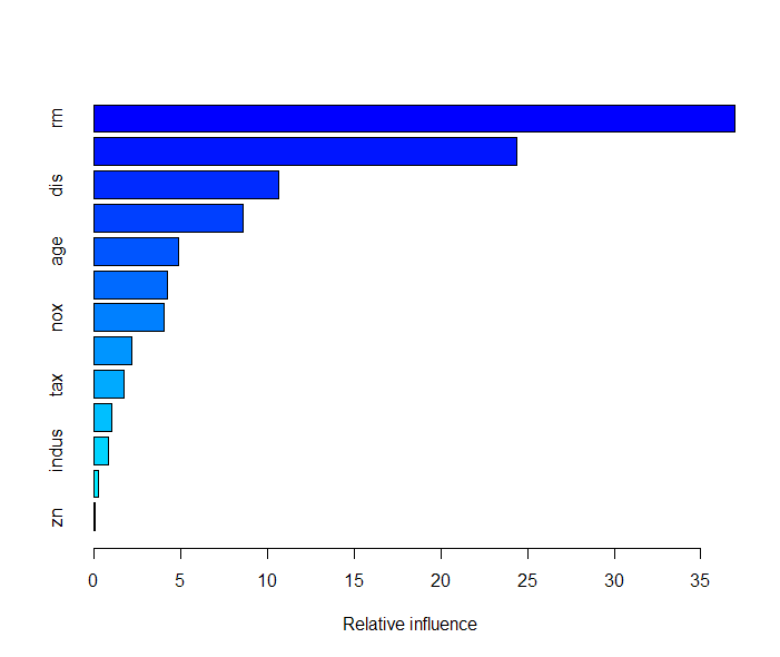
The summary of the Model gives a feature importance plot.In the above list is on the top is the most important variable and at last is the least important variable.
And the 2 most important features which explain the maximum variance in the Data set is lstat i.e lower status of the population (percent) and rm which is average number of rooms per dwelling.
Variable importance plot–
Plotting the Partial Dependence Plot
The partial Dependence Plots will tell us the relationship and dependence of the variables \(X_i\) with the Response variable \(Y\).
#Plot of Response variable with lstat variable
plot(Boston.boost,i="lstat")
#Inverse relation with lstat variable

plot(Boston.boost,i="rm")
#as the average number of rooms increases the the price increases
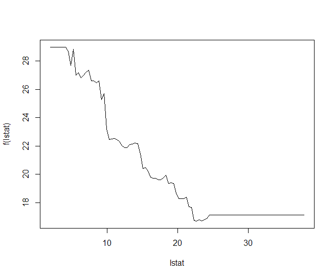
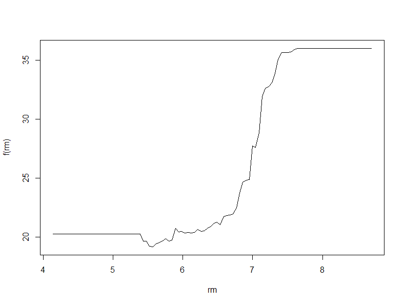
The above plot simply shows the relation between the variables in the x-axis and the mapping function \(f(x)\) on the y-axis.First plot shows that lstat is negatively correlated with the response mdev, whereas the second one shows that rm is somewhat directly related to mdev.
cor(Boston$lstat,Boston$medv)#negetive correlation coeff-r

cor(Boston$rm,Boston$medv)#positive correlation coeff-r

> cor(Boston$lstat,Boston$medv)
[1] -0.7376627

> cor(Boston$rm,Boston$medv)
[1] 0.6953599
Prediction on Test Set
We will compute the Test Error as a function of number of Trees.
n.trees = seq(from=100 ,to=10000, by=100) #no of trees-a vector of 100 values

#Generating a Prediction matrix for each Tree
predmatrix<-predict(Boston.boost,Boston[-train,],n.trees = n.trees)
dim(predmatrix) #dimentions of the Prediction Matrix

#Calculating The Mean squared Test Error
test.error<-with(Boston[-train,],apply( (predmatrix-medv)^2,2,mean))
head(test.error) #contains the Mean squared test error for each of the 100 trees averaged

#Plotting the test error vs number of trees

plot(n.trees , test.error , pch=19,col="blue",xlab="Number of Trees",ylab="Test Error", main = "Perfomance of Boosting on Test Set")

#adding the RandomForests Minimum Error line trained on same data and similar parameters
abline(h = min(test.err),col="red") #test.err is the test error of a Random forest fitted on same data
legend("topright",c("Minimum Test error Line for Random Forests"),col="red",lty=1,lwd=1)


dim(predmatrix)
[1] 206 100

head(test.error)
      100       200       300       400       500       600
26.428346 14.938232 11.232557  9.221813  7.873472  6.911313
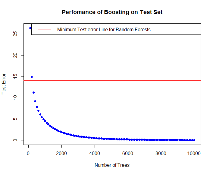
In the above plot the red line represents the least error obtained from training a Random forest with same data and same parameters and number of trees.Boosting outperforms Random Forests on same test dataset with lesser Mean squared Test Errors.
Other Useful resource
One of the most amazing courses out there on Gradient Boosting and essentials of Tree based modelling is this Ensemble Learning and Tree based modelling in R. This one is my personal favorite as it has helped me a lot to understand ensemble learning properly and tree based modelling techniques. So I do insist the readers to try out and complete this amazing course.
Conclusion
From the above plot we can notice that if boosting is done properly by selecting appropriate tuning parameters such as shrinkage parameter \(lambda\) ,the number of splits we want and the number of trees \(n\), then it can generalize really well and convert a weak learner to strong learner. Ensembling techniques are really well and tend to outperform a single learner which is prone to either overfitting or underfitting or generate thousands or hundreds of them,then combine them to produce a better and stronger model.
Hope you guys liked the article, make sure to like and share. Cheers!!.