ARIMA Modeling
AutoRegressive Integrated Moving Average
Install Packages
library(readxl)
library(lmtest)
library(forecast)
library(FitAR)
library(fUnitRoots)
Import Data Set
table2 <- read_excel("Datum/1 SCOPUS/2022/Feb-01/Data/table2.xlsx",sheet = "Sheet2")
View(table2)
summary(table2)
    avg_jual        avg_beli
 Min.   : 8808   Min.   : 8766
 1st Qu.:13498   1st Qu.:13480
 Median :14190   Median :14078
 Mean   :13979   Mean   :13800
 3rd Qu.:14705   3rd Qu.:14257
 Max.   :15753   Max.   :15020
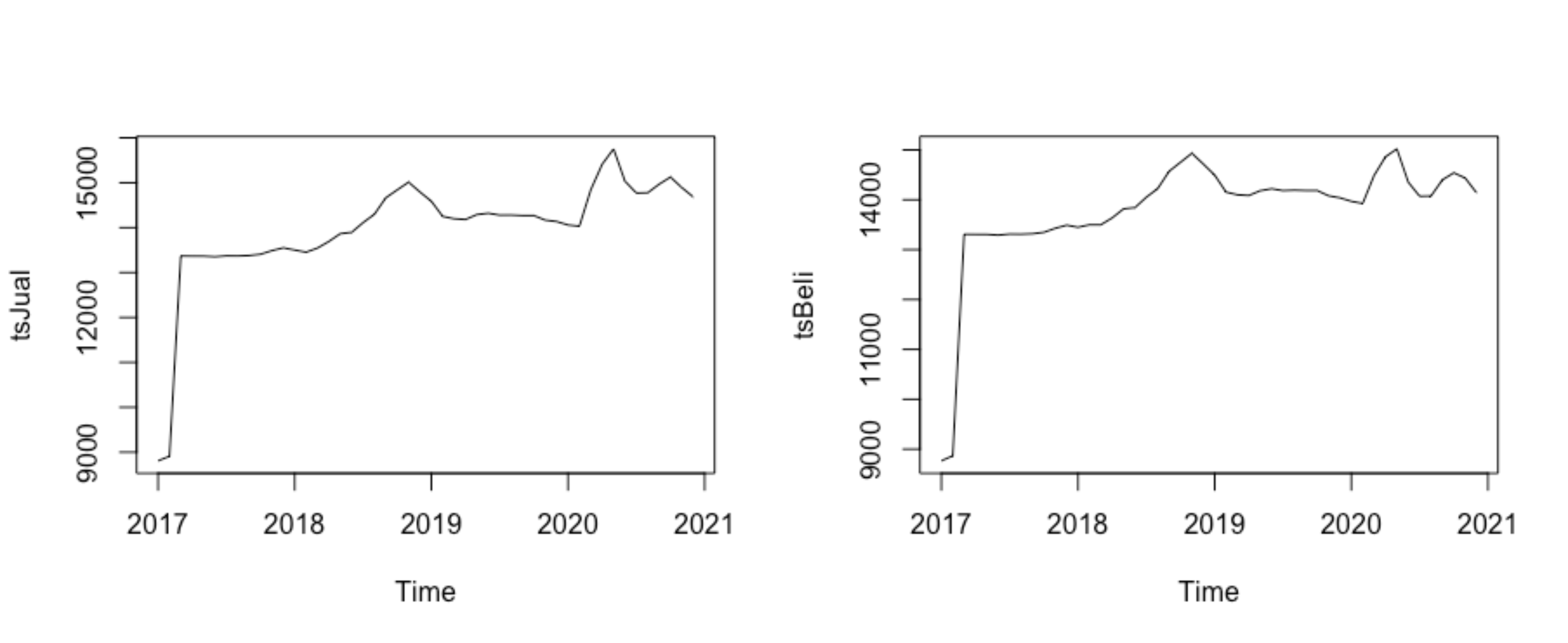
tsJual = ts(table2$avg_jual, start = c(2017,1), frequency = 12)
plot(tsJual)
tsBeli = ts(table2$avg_beli, start = c(2017,1), frequency = 12)
plot(tsBeli)
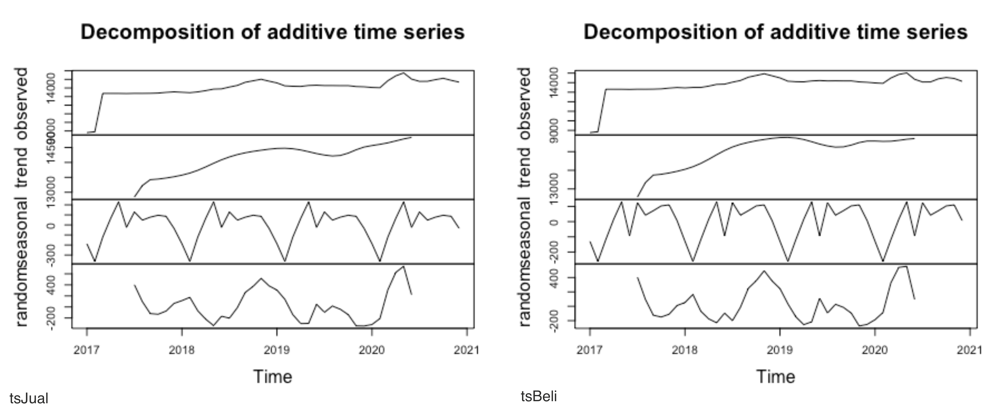
components.tsJual = decompose(tsJual)
plot(components.tsJual)
components.tsBeli = decompose(tsBeli)
plot(components.tsBeli)
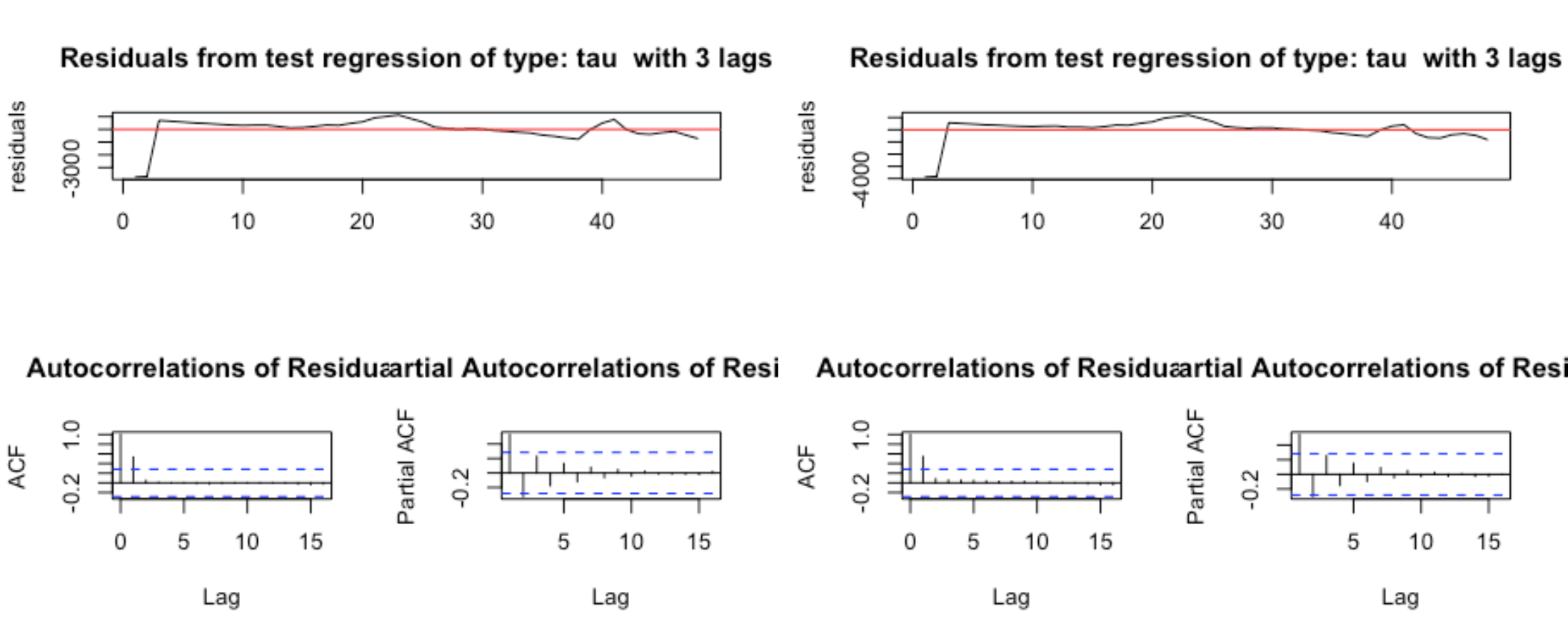
urkpssTest(tsJual, type = c("tau"), lags = c("short"),use.lag = NULL, doplot = TRUE)
urkpssTest(tsBeli, type = c("tau"), lags = c("short"),use.lag = NULL, doplot = TRUE)
sstationary_Jual = diff(tsJual, differences=1)
plot(tsstationary_Jual)
tsstationary_Beli = diff(tsBeli, differences=1)
plot(tsstationary_Beli)
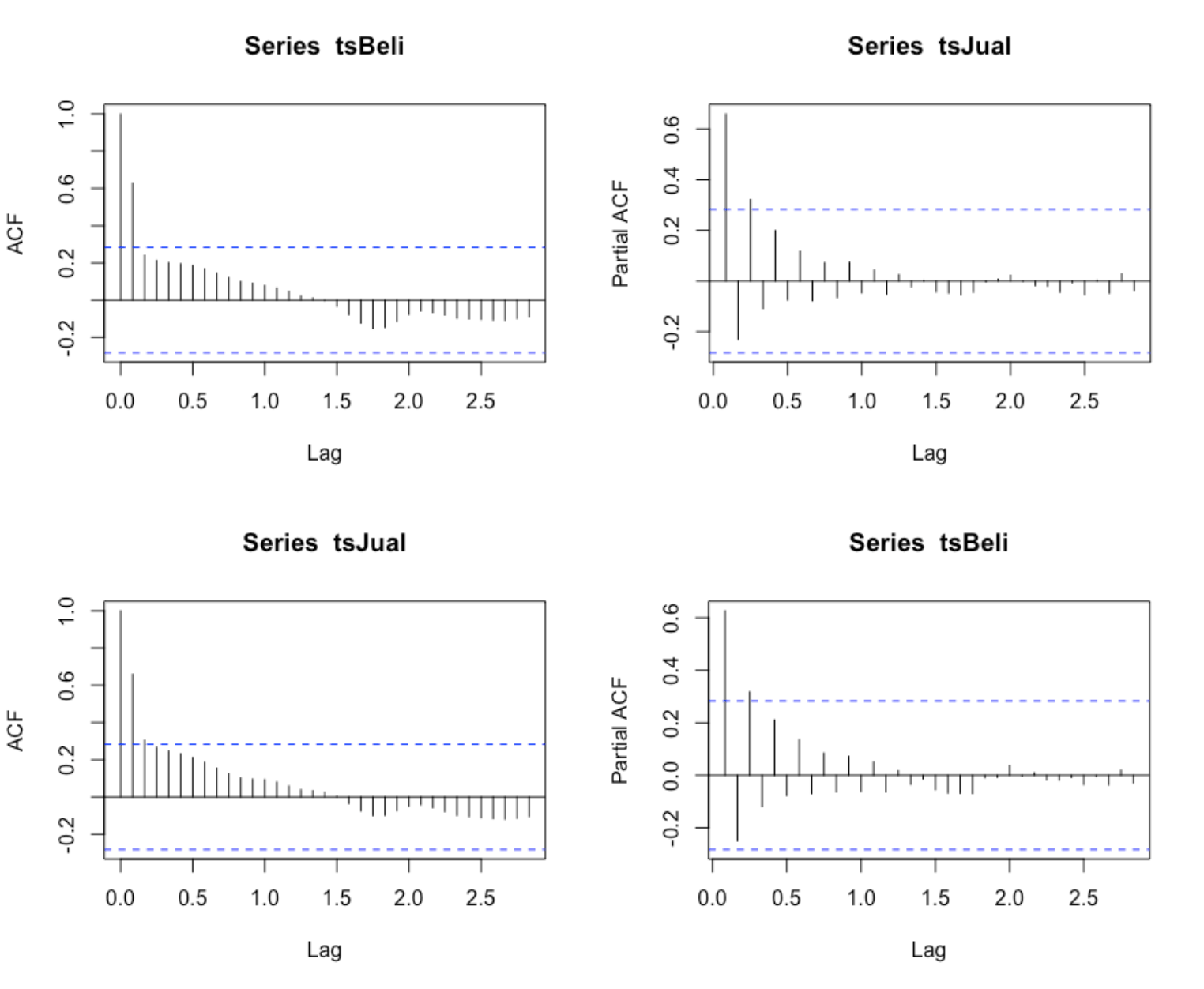
acf(tsJual,lag.max=34)
acf(tsBeli,lag.max=34)
Pacf(tsJual,lag.max=34)
Pacf(tsBeli,lag.max=34)
timeseriesseasonallyadjusted_Jual <- tsJual- components.tsJual$seasonal
tsstationary_Jual <- diff(timeseriesseasonallyadjusted_Jual, differences=1)
timeseriesseasonallyadjusted_Beli <- tsJual- components.tsBeli$seasonal
tsstationary_Beli <- diff(timeseriesseasonallyadjusted_Beli, differences=1)
plot(timeseriesseasonallyadjusted_Beli)
plot(timeseriesseasonallyadjusted_Jual)
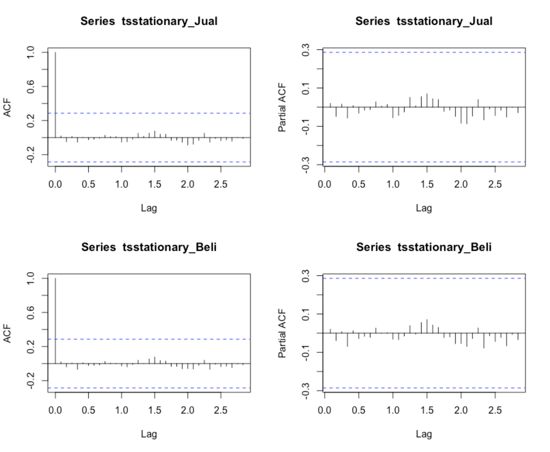
acf(tsstationary_Jual, lag.max=34)
pacf(tsstationary_Jual, lag.max=34)
acf(tsstationary_Beli, lag.max=34)
pacf(tsstationary_Beli, lag.max=34)
fitARIMA_Jual <- arima(tsJual, order=c(1,1,1),seasonal = list(order = c(1,0,0), period = 12),method="ML")
fitARIMA_Beli <- arima(tsBeli, order=c(1,1,1),seasonal = list(order = c(1,0,0), period = 12),method="ML")
coeftest(fitARIMA_Jual)
z test of coefficients:

      Estimate Std. Error z value Pr(>|z|)
ar1  -0.021344   1.837953 -0.0116   0.9907
ma1   0.083561   1.842706  0.0453   0.9638
sar1  0.072859   0.274394  0.2655   0.7906
coeftest(fitARIMA_Beli)
z test of coefficients:

       Estimate Std. Error z value Pr(>|z|)
ar1   0.0032167  0.6907733  0.0047   0.9963
ma1   0.0509199  0.7058832  0.0721   0.9425
sar1 -0.0026367  0.3522116 -0.0075   0.9940
fitARIMA_Jual
Call:
arima(x = tsJual, order = c(1, 1, 1), seasonal = list(order = c(1, 0, 0), period = 12),
    method = "ML")

Coefficients:
          ar1     ma1    sar1
      -0.0213  0.0836  0.0729
s.e.   1.8380  1.8427  0.2744

sigma^2 estimated as 472215:  log likelihood = -373.76,  aic = 755.51
fitARIMA_Beli
Call:
arima(x = tsBeli, order = c(1, 1, 1), seasonal = list(order = c(1, 0, 0), period = 12),
    method = "ML")

Coefficients:
         ar1     ma1     sar1
      0.0032  0.0509  -0.0026
s.e.  0.6908  0.7059   0.3522

sigma^2 estimated as 457012:  log likelihood = -372.95,  aic = 753.91
confint(fitARIMA_Beli)
 2.5 %    97.5 %
ar1  -1.3506740 1.3571074
ma1  -1.3325858 1.4344256
sar1 -0.6929589 0.6876854
confint(fitARIMA_Jual)
2.5 %    97.5 %
ar1  -3.6236644 3.5809772
ma1  -3.5280769 3.6951992
sar1 -0.4649435 0.6106622
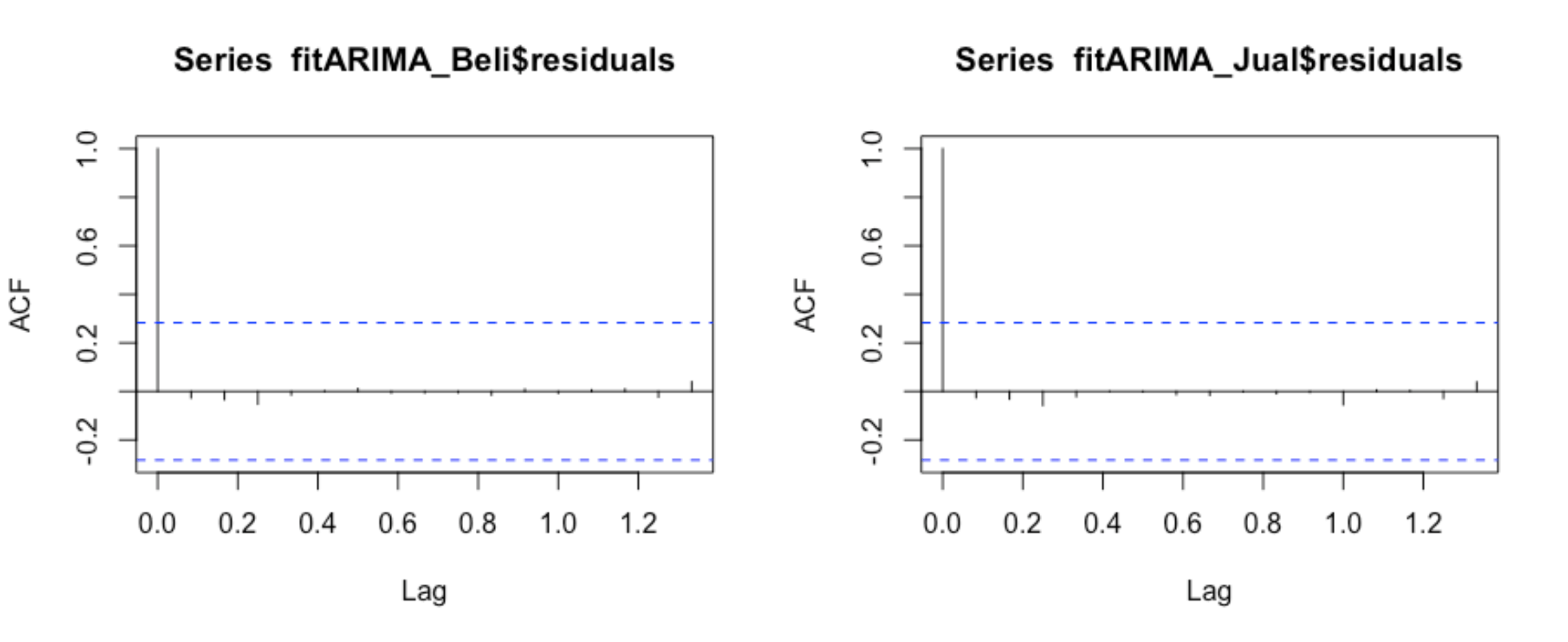
acf(fitARIMA_Beli$residuals)
acf(fitARIMA_Jual$residuals)
boxplot(fitARIMA_Jual$residuals,k=2,StartLag=1)
LjungBoxTest(fitARIMA_Jual$residuals,k=2,StartLag=1)
boxplot(fitARIMA_Beli$residuals,k=2,StartLag=1)
LjungBoxTest(fitARIMA_Beli$residuals,k=2,StartLag=1)
qqnorm(fitARIMA_Jual$residuals)
qqline(fitARIMA_Jual$residuals)
qqnorm(fitARIMA_Beli$residuals)
qqline(fitARIMA_Beli$residuals)
arima(tsJual)
Call:
arima(x = tsJual)

Coefficients:
       intercept
      13978.5625
s.e.    177.7277

sigma^2 estimated as 1516180:  log likelihood = -409.67,  aic = 823.34
arima(tsBeli)
Call:
arima(x = tsBeli)

Coefficients:
       intercept
      13800.3958
s.e.    165.1939

sigma^2 estimated as 1309870:  log likelihood = -406.16,  aic = 816.32
auto.arima(tsJual, trace=TRUE)
ARIMA(2,1,2)(1,0,1)[12] with drift         : Inf
 ARIMA(0,1,0)            with drift         : 750.4713
 ARIMA(1,1,0)(1,0,0)[12] with drift         : 755.0944
 ARIMA(0,1,1)(0,0,1)[12] with drift         : 755.0899
 ARIMA(0,1,0)                               : 749.8579
 ARIMA(0,1,0)(1,0,0)[12] with drift         : 752.7432
 ARIMA(0,1,0)(0,0,1)[12] with drift         : 752.7402
 ARIMA(0,1,0)(1,0,1)[12] with drift         : Inf
 ARIMA(1,1,0)            with drift         : 752.7152
 ARIMA(0,1,1)            with drift         : 752.7136
 ARIMA(1,1,1) with drift         : Inf

 Best model: ARIMA(0,1,0)

Series: tsJual
ARIMA(0,1,0)

sigma^2 = 475492:  log likelihood = -373.88
AIC=749.77   AICc=749.86   BIC=751.62
auto.arima(tsBeli, trace=TRUE)
ARIMA(2,1,2)(1,0,1)[12] with drift         : Inf
 ARIMA(0,1,0)            with drift         : 748.9614
 ARIMA(1,1,0)(1,0,0)[12] with drift         : 753.5961
 ARIMA(0,1,1)(0,0,1)[12] with drift         : 753.5933
 ARIMA(0,1,0)                               : 748.1365
 ARIMA(0,1,0)(1,0,0)[12] with drift         : 751.2314
 ARIMA(0,1,0)(0,0,1)[12] with drift         : 751.2295
 ARIMA(0,1,0)(1,0,1)[12] with drift         : 753.6222
 ARIMA(1,1,0)            with drift         : 751.2183
 ARIMA(0,1,1)            with drift         : 751.2173
 ARIMA(1,1,1) with drift         : Inf

 Best model: ARIMA(0,1,0)

Series: tsBeli
ARIMA(0,1,0)

sigma^2 = 458392:  log likelihood = -373.02
AIC=748.05   AICc=748.14   BIC=749.9
fitARIMA_Jual
Call:
arima(x = tsJual, order = c(1, 1, 1), seasonal = list(order = c(1, 0, 0), period = 12),
    method = "ML")

Coefficients:
          ar1     ma1    sar1
      -0.0213  0.0836  0.0729
s.e.   1.8380  1.8427  0.2744

sigma^2 estimated as 472215:  log likelihood = -373.76,  aic = 755.51
fitARIMA_Beli
all:
arima(x = tsBeli, order = c(1, 1, 1), seasonal = list(order = c(1, 0, 0), period = 12),
    method = "ML")

Coefficients:
         ar1     ma1     sar1
      0.0032  0.0509  -0.0026
s.e.  0.6908  0.7059   0.3522

sigma^2 estimated as 457012:  log likelihood = -372.95,  aic = 753.91
predict(fitARIMA_Jual,n.ahead = 1)
$pred
         Jan
2021 14665.9

$se
          Jan
2021 687.1792
predict(fitARIMA_Beli,n.ahead = 1)
$pred
          Jan
2021 14122.35

$se
          Jan
2021 676.0263
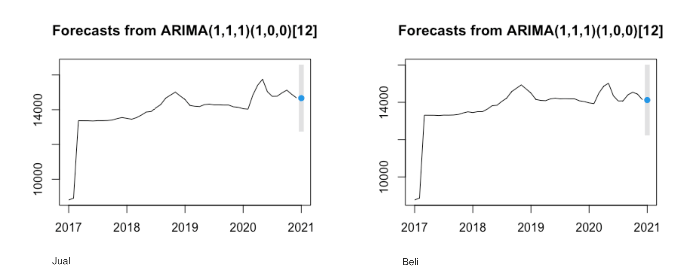
futurVal_Beli <- forecast(fitARIMA_Beli,h=1, level=c(99.5))
futurVal_Jual <- forecast(fitARIMA_Jual,h=1, level=c(99.5))
plot(futurVal_Beli)
plot(futurVal_Jual)
summary(futurVal_Jual)
Forecast method: ARIMA(1,1,1)(1,0,0)[12]

Model Information:

Call:
arima(x = tsJual, order = c(1, 1, 1), seasonal = list(order = c(1, 0, 0), period = 12),
    method = "ML")

Coefficients:
          ar1     ma1    sar1
      -0.0213  0.0836  0.0729
s.e.   1.8380  1.8427  0.2744

sigma^2 estimated as 472215:  log likelihood = -373.76,  aic = 755.51

Error measures:
                   ME     RMSE      MAE      MPE     MAPE      MASE        ACF1
Training set 107.4817 679.9846 237.3794 0.794616 1.695755 0.2583878 -0.02594214

Forecasts:
         Point Forecast  Lo 99.5  Hi 99.5
Jan 2021        14665.9 12736.97 16594.84
summary(futurVal_Beli)
Forecast method: ARIMA(1,1,1)(1,0,0)[12]

Model Information:

Call:
arima(x = tsBeli, order = c(1, 1, 1), seasonal = list(order = c(1, 0, 0), period = 12),
    method = "ML")

Coefficients:
         ar1     ma1     sar1
      0.0032  0.0509  -0.0026
s.e.  0.6908  0.7059   0.3522

sigma^2 estimated as 457012:  log likelihood = -372.95,  aic = 753.91

Error measures:
                  ME     RMSE      MAE       MPE     MAPE      MASE        ACF1
Training set 106.293 668.9485 220.1657 0.7954476 1.599417 0.2807839 -0.02688605

Forecasts:
         Point Forecast  Lo 99.5  Hi 99.5
Jan 2021       14122.35 12224.72 16019.98