Customer churn occurs when customers or subscribers stop doing business with a company or service, also known as customer attrition. It is also referred as loss of clients or customers. One industry in which churn rates are particularly useful is the telecommunications industry, because most customers have multiple options from which to choose within a geographic location.
Similar concept with predicting employee turnover, we are going to predict customer churn using telecom dataset. We will introduce Logistic Regression, Decision Tree, and Random Forest. But this time, we will do all of the above in R. Let’s get started!
Data Preprocessing
The data was downloaded from IBM Sample Data Sets. Each row represents a customer, each column contains that customer’s attributes:
library(plyr)
library(corrplot)
library(ggplot2)
library(gridExtra)
library(ggthemes)
library(caret)
library(MASS)
library(randomForest)
library(party)

churn <- read.csv('Telco-Customer-Churn.csv')
str(churn)
'data.frame':	7043 obs. of  21 variables:
 $ customerID      : Factor w/ 7043 levels "0002-ORFBO","0003-MKNFE",..: 5376 3963 2565 5536 6512 6552 1003 4771 5605 4535 ...
 $ gender          : Factor w/ 2 levels "Female","Male": 1 2 2 2 1 1 2 1 1 2 ...
 $ SeniorCitizen   : int  0 0 0 0 0 0 0 0 0 0 ...
 $ Partner         : Factor w/ 2 levels "No","Yes": 2 1 1 1 1 1 1 1 2 1 ...
 $ Dependents      : Factor w/ 2 levels "No","Yes": 1 1 1 1 1 1 2 1 1 2 ...
 $ tenure          : int  1 34 2 45 2 8 22 10 28 62 ...
 $ PhoneService    : Factor w/ 2 levels "No","Yes": 1 2 2 1 2 2 2 1 2 2 ...
 $ MultipleLines   : Factor w/ 3 levels "No","No phone service",..: 2 1 1 2 1 3 3 2 3 1 ...
 $ InternetService : Factor w/ 3 levels "DSL","Fiber optic",..: 1 1 1 1 2 2 2 1 2 1 ...
 $ OnlineSecurity  : Factor w/ 3 levels "No","No internet service",..: 1 3 3 3 1 1 1 3 1 3 ...
 $ OnlineBackup    : Factor w/ 3 levels "No","No internet service",..: 3 1 3 1 1 1 3 1 1 3 ...
 $ DeviceProtection: Factor w/ 3 levels "No","No internet service",..: 1 3 1 3 1 3 1 1 3 1 ...
 $ TechSupport     : Factor w/ 3 levels "No","No internet service",..: 1 1 1 3 1 1 1 1 3 1 ...
 $ StreamingTV     : Factor w/ 3 levels "No","No internet service",..: 1 1 1 1 1 3 3 1 3 1 ...
 $ StreamingMovies : Factor w/ 3 levels "No","No internet service",..: 1 1 1 1 1 3 1 1 3 1 ...
 $ Contract        : Factor w/ 3 levels "Month-to-month",..: 1 2 1 2 1 1 1 1 1 2 ...
 $ PaperlessBilling: Factor w/ 2 levels "No","Yes": 2 1 2 1 2 2 2 1 2 1 ...
 $ PaymentMethod   : Factor w/ 4 levels "Bank transfer (automatic)",..: 3 4 4 1 3 3 2 4 3 1 ...
 $ MonthlyCharges  : num  29.9 57 53.9 42.3 70.7 ...
 $ TotalCharges    : num  29.9 1889.5 108.2 1840.8 151.7 ...
 $ Churn           : Factor w/ 2 levels "No","Yes": 1 1 2 1 2 2 1 1 2 1 ...
The raw data contains 7043 rows (customers) and 21 columns (features). The “Churn” column is our target.
We use sapply to check the number if missing values in each columns. We found that there are 11 missing values in “TotalCharges” columns. So, let’s remove all rows with missing values.
sapply(churn, function(x) sum(is.na(x)))
customerID           gender    SeniorCitizen          Partner
               0                0                0                0
      Dependents           tenure     PhoneService    MultipleLines
               0                0                0                0
 InternetService   OnlineSecurity     OnlineBackup DeviceProtection
               0                0                0                0
     TechSupport      StreamingTV  StreamingMovies         Contract
               0                0                0                0
PaperlessBilling    PaymentMethod   MonthlyCharges     TotalCharges
               0                0                0               11
           Churn
               0
churn <- churn[complete.cases(churn), ]
Look at the variables, we can see that we have some wranglings to do.
1. We will change “No internet service” to “No” for six columns, they are: “OnlineSecurity”, “OnlineBackup”, “DeviceProtection”, “TechSupport”, “streamingTV”, “streamingMovies”.
cols_recode1 <- c(10:15)
for(i in 1:ncol(churn[,cols_recode1])) {
        churn[,cols_recode1][,i] <- as.factor(mapvalues
                                              (churn[,cols_recode1][,i], from =c("No internet service"),to=c("No")))
}
2. We will change “No phone service” to “No” for column “MultipleLines”
churn$MultipleLines <- as.factor(mapvalues(churn$MultipleLines,
                                           from=c("No phone service"),
                                           to=c("No")))
3. Since the minimum tenure is 1 month and maximum tenure is 72 months, we can group them into five tenure groups: “0–12 Month”, “12–24 Month”, “24–48 Months”, “48–60 Month”, “> 60 Month”
min(churn$tenure); max(churn$tenure)
[1] 1
[1] 72
group_tenure = 0 & tenure  12 & tenure  24 & tenure  48 & tenure  60){
        return('> 60 Month')
    }
}
churn$tenure_group <- sapply(churn$tenure,group_tenure)
churn$tenure_group <- as.factor(churn$tenure_group)
4. Change the values in column “SeniorCitizen” from 0 or 1 to “No” or “Yes”.
churn$SeniorCitizen <- as.factor(mapvalues(churn$SeniorCitizen,
                                      from=c("0","1"),
                                      to=c("No", "Yes")))
5. Remove the columns we do not need for the analysis.
churn$customerID <- NULL
churn$tenure <- NULL
Exploratory data analysis and feature selection
Correlation between numeric variables
numeric.var <- sapply(churn, is.numeric)
corr.matrix <- cor(churn[,numeric.var])
corrplot(corr.matrix, main="\n\nCorrelation Plot for Numerical Variables", method="number")
Gives this plot:
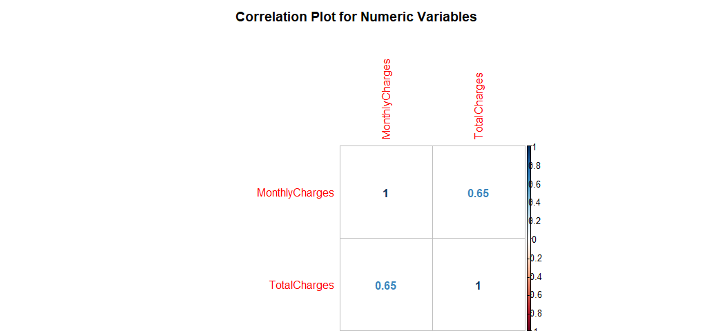
The Monthly Charges and Total Charges are correlated. So one of them will be removed from the model. We remove Total Charges.
churn$TotalCharges <- NULL
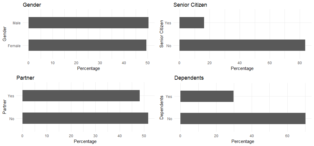
Bar plots of categorical variables
p1 <- ggplot(churn, aes(x=gender)) + ggtitle("Gender") + xlab("Gender") +
  geom_bar(aes(y = 100*(..count..)/sum(..count..)), width = 0.5) + ylab("Percentage") + coord_flip() + theme_minimal()
p2 <- ggplot(churn, aes(x=SeniorCitizen)) + ggtitle("Senior Citizen") + xlab("Senior Citizen") +
  geom_bar(aes(y = 100*(..count..)/sum(..count..)), width = 0.5) + ylab("Percentage") + coord_flip() + theme_minimal()
p3 <- ggplot(churn, aes(x=Partner)) + ggtitle("Partner") + xlab("Partner") +
  geom_bar(aes(y = 100*(..count..)/sum(..count..)), width = 0.5) + ylab("Percentage") + coord_flip() + theme_minimal()
p4 <- ggplot(churn, aes(x=Dependents)) + ggtitle("Dependents") + xlab("Dependents") +
  geom_bar(aes(y = 100*(..count..)/sum(..count..)), width = 0.5) + ylab("Percentage") + coord_flip() + theme_minimal()
grid.arrange(p1, p2, p3, p4, ncol=2)
Gives this plot:
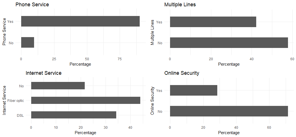
p5 <- ggplot(churn, aes(x=PhoneService)) + ggtitle("Phone Service") + xlab("Phone Service") +
  geom_bar(aes(y = 100*(..count..)/sum(..count..)), width = 0.5) + ylab("Percentage") + coord_flip() + theme_minimal()
p6 <- ggplot(churn, aes(x=MultipleLines)) + ggtitle("Multiple Lines") + xlab("Multiple Lines") +
  geom_bar(aes(y = 100*(..count..)/sum(..count..)), width = 0.5) + ylab("Percentage") + coord_flip() + theme_minimal()
p7 <- ggplot(churn, aes(x=InternetService)) + ggtitle("Internet Service") + xlab("Internet Service") +
  geom_bar(aes(y = 100*(..count..)/sum(..count..)), width = 0.5) + ylab("Percentage") + coord_flip() + theme_minimal()
p8 <- ggplot(churn, aes(x=OnlineSecurity)) + ggtitle("Online Security") + xlab("Online Security") +
  geom_bar(aes(y = 100*(..count..)/sum(..count..)), width = 0.5) + ylab("Percentage") + coord_flip() + theme_minimal()
grid.arrange(p5, p6, p7, p8, ncol=2)
Gives this plot:
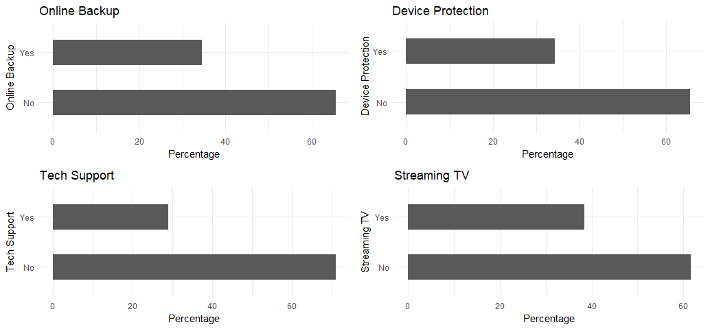
p9 <- ggplot(churn, aes(x=OnlineBackup)) + ggtitle("Online Backup") + xlab("Online Backup") +
  geom_bar(aes(y = 100*(..count..)/sum(..count..)), width = 0.5) + ylab("Percentage") + coord_flip() + theme_minimal()
p10 <- ggplot(churn, aes(x=DeviceProtection)) + ggtitle("Device Protection") + xlab("Device Protection") +
  geom_bar(aes(y = 100*(..count..)/sum(..count..)), width = 0.5) + ylab("Percentage") + coord_flip() + theme_minimal()
p11 <- ggplot(churn, aes(x=TechSupport)) + ggtitle("Tech Support") + xlab("Tech Support") +
  geom_bar(aes(y = 100*(..count..)/sum(..count..)), width = 0.5) + ylab("Percentage") + coord_flip() + theme_minimal()
p12 <- ggplot(churn, aes(x=StreamingTV)) + ggtitle("Streaming TV") + xlab("Streaming TV") +
  geom_bar(aes(y = 100*(..count..)/sum(..count..)), width = 0.5) + ylab("Percentage") + coord_flip() + theme_minimal()
grid.arrange(p9, p10, p11, p12, ncol=2)
Gives this plot:
p13 <- ggplot(churn, aes(x=StreamingMovies)) + ggtitle("Streaming Movies") + xlab("Streaming Movies") +
  geom_bar(aes(y = 100*(..count..)/sum(..count..)), width = 0.5) + ylab("Percentage") + coord_flip() + theme_minimal()
p14 <- ggplot(churn, aes(x=Contract)) + ggtitle("Contract") + xlab("Contract") +
  geom_bar(aes(y = 100*(..count..)/sum(..count..)), width = 0.5) + ylab("Percentage") + coord_flip() + theme_minimal()
p15 <- ggplot(churn, aes(x=PaperlessBilling)) + ggtitle("Paperless Billing") + xlab("Paperless Billing") +
  geom_bar(aes(y = 100*(..count..)/sum(..count..)), width = 0.5) + ylab("Percentage") + coord_flip() + theme_minimal()
p16 <- ggplot(churn, aes(x=PaymentMethod)) + ggtitle("Payment Method") + xlab("Payment Method") +
  geom_bar(aes(y = 100*(..count..)/sum(..count..)), width = 0.5) + ylab("Percentage") + coord_flip() + theme_minimal()
p17 <- ggplot(churn, aes(x=tenure_group)) + ggtitle("Tenure Group") + xlab("Tenure Group") +
  geom_bar(aes(y = 100*(..count..)/sum(..count..)), width = 0.5) + ylab("Percentage") + coord_flip() + theme_minimal()
grid.arrange(p13, p14, p15, p16, p17, ncol=2)
Gives this plot:
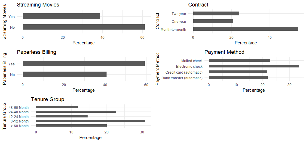
All of the categorical variables seem to have a reasonably broad distribution, therefore, all of them will be kept for the further analysis.
Logistic Regression
First, we split the data into training and testing sets
intrain<- createDataPartition(churn$Churn,p=0.7,list=FALSE)
set.seed(2017)
training<- churn[intrain,]
testing<- churn[-intrain,]
Confirm the splitting is correct
dim(training); dim(testing)
[1] 4924   19
[1] 2108   19
Fitting the Logistic Regression Model
LogModel <- glm(Churn ~ .,family=binomial(link="logit"),data=training)
print(summary(LogModel))
Call:
glm(formula = Churn ~ ., family = binomial(link = "logit"), data = training)

Deviance Residuals:
    Min       1Q   Median       3Q      Max
-2.0370  -0.6793  -0.2861   0.6590   3.1608

Coefficients:
                                      Estimate Std. Error z value Pr(>|z|)
(Intercept)                          -2.030149   1.008223  -2.014 0.044053 *
genderMale                           -0.039006   0.077686  -0.502 0.615603
SeniorCitizenYes                      0.194408   0.101151   1.922 0.054611 .
PartnerYes                           -0.062031   0.092911  -0.668 0.504363
DependentsYes                        -0.017974   0.107659  -0.167 0.867405
PhoneServiceYes                      -0.387097   0.788745  -0.491 0.623585
MultipleLinesYes                      0.345052   0.214799   1.606 0.108187
InternetServiceFiber optic            1.022836   0.968062   1.057 0.290703
InternetServiceNo                    -0.829521   0.978909  -0.847 0.396776
OnlineSecurityYes                    -0.393647   0.215993  -1.823 0.068379 .
OnlineBackupYes                      -0.113220   0.213825  -0.529 0.596460
DeviceProtectionYes                  -0.025797   0.213317  -0.121 0.903744
TechSupportYes                       -0.306423   0.220920  -1.387 0.165433
StreamingTVYes                        0.399209   0.395912   1.008 0.313297
StreamingMoviesYes                    0.338852   0.395890   0.856 0.392040
ContractOne year                     -0.805584   0.127125  -6.337 2.34e-10 ***
ContractTwo year                     -1.662793   0.216346  -7.686 1.52e-14 ***
PaperlessBillingYes                   0.338724   0.089407   3.789 0.000152 ***
PaymentMethodCredit card (automatic) -0.018574   0.135318  -0.137 0.890826
PaymentMethodElectronic check         0.373214   0.113029   3.302 0.000960 ***
PaymentMethodMailed check             0.001400   0.136446   0.010 0.991815
MonthlyCharges                       -0.005001   0.038558  -0.130 0.896797
tenure_group0-12 Month                1.858899   0.205956   9.026  < 2e-16 ***
tenure_group12-24 Month               0.968497   0.201452   4.808 1.53e-06 ***
tenure_group24-48 Month               0.574822   0.185500   3.099 0.001943 **
tenure_group48-60 Month               0.311790   0.200096   1.558 0.119185
---
Signif. codes:  0 ‘***’ 0.001 ‘**’ 0.01 ‘*’ 0.05 ‘.’ 0.1 ‘ ’ 1

(Dispersion parameter for binomial family taken to be 1)

    Null deviance: 5702.8  on 4923  degrees of freedom
Residual deviance: 4094.4  on 4898  degrees of freedom
AIC: 4146.4

Number of Fisher Scoring iterations: 6
Feature Analysis
The top three most-relevant features include Contract, tenure_group and PaperlessBilling.
anova(LogModel, test="Chisq")
Analysis of Deviance Table
Model: binomial, link: logit
Response: Churn
Terms added sequentially (first to last)
                 Df Deviance Resid. Df Resid. Dev  Pr(>Chi)
NULL                              4923     5702.8
gender            1     0.39      4922     5702.4 0.5318602
SeniorCitizen     1    95.08      4921     5607.3 < 2.2e-16 ***
Partner           1   107.29      4920     5500.0 < 2.2e-16 ***
Dependents        1    27.26      4919     5472.7 1.775e-07 ***
PhoneService      1     1.27      4918     5471.5 0.2597501
MultipleLines     1     9.63      4917     5461.8 0.0019177 **
InternetService   2   452.01      4915     5009.8 < 2.2e-16 ***
OnlineSecurity    1   183.83      4914     4826.0 < 2.2e-16 ***
OnlineBackup      1    69.94      4913     4756.1 < 2.2e-16 ***
DeviceProtection  1    47.58      4912     4708.5 5.287e-12 ***
TechSupport       1    82.78      4911     4625.7 < 2.2e-16 ***
StreamingTV       1     4.90      4910     4620.8 0.0269174 *
StreamingMovies   1     0.36      4909     4620.4 0.5461056
Contract          2   309.25      4907     4311.2 < 2.2e-16 ***
PaperlessBilling  1    14.21      4906     4297.0 0.0001638 ***
PaymentMethod     3    38.85      4903     4258.1 1.867e-08 ***
MonthlyCharges    1     0.10      4902     4258.0 0.7491553
tenure_group      4   163.67      4898     4094.4 < 2.2e-16 ***
---
Signif. codes:  0 ‘***’ 0.001 ‘**’ 0.01 ‘*’ 0.05 ‘.’ 0.1 ‘ ’ 1
Analyzing the deviance table we can see the drop in deviance when adding each variable one at a time. Adding InternetService, Contract and tenure_group significantly reduces the residual deviance. The other variables such as PaymentMethod and Dependents seem to improve the model less even though they all have low p-values.
Assessing the predictive ability of the Logistic Regression model
testing$Churn <- as.character(testing$Churn)
testing$Churn[testing$Churn=="No"] <- "0"
testing$Churn[testing$Churn=="Yes"] <- "1"
fitted.results <- predict(LogModel,newdata=testing,type='response')
fitted.results  0.5,1,0)
misClasificError <- mean(fitted.results != testing$Churn)
print(paste('Logistic Regression Accuracy',1-misClasificError))
[1] "Logistic Regression Accuracy 0.796489563567362"
Logistic Regression Confusion Matrix
print("Confusion Matrix for Logistic Regression"); table(testing$Churn, fitted.results > 0.5)
[1] "Confusion Matrix for Logistic Regression"

    FALSE TRUE
  0  1392  156
  1   273  287
Odds Ratio
One of the interesting performance measurements in logistic regression is Odds Ratio.Basically, Odds ratio is what the odds of an event is happening.
exp(cbind(OR=coef(LogModel), confint(LogModel)))
Waiting for profiling to be done...
                                            OR      2.5 %     97.5 %
(Intercept)                          0.1313160 0.01815817  0.9461855
genderMale                           0.9617454 0.82587632  1.1199399
SeniorCitizenYes                     1.2145919 0.99591418  1.4807053
PartnerYes                           0.9398537 0.78338071  1.1276774
DependentsYes                        0.9821863 0.79488224  1.2124072
PhoneServiceYes                      0.6790251 0.14466019  3.1878587
MultipleLinesYes                     1.4120635 0.92707245  2.1522692
InternetServiceFiber optic           2.7810695 0.41762316 18.5910286
InternetServiceNo                    0.4362582 0.06397364  2.9715699
OnlineSecurityYes                    0.6745919 0.44144273  1.0296515
OnlineBackupYes                      0.8929545 0.58709919  1.3577947
DeviceProtectionYes                  0.9745328 0.64144877  1.4805460
TechSupportYes                       0.7360754 0.47707096  1.1344691
StreamingTVYes                       1.4906458 0.68637788  3.2416264
StreamingMoviesYes                   1.4033353 0.64624171  3.0518161
ContractOne year                     0.4468271 0.34725066  0.5717469
ContractTwo year                     0.1896086 0.12230199  0.2861341
PaperlessBillingYes                  1.4031556 1.17798691  1.6725920
PaymentMethodCredit card (automatic) 0.9815977 0.75273387  1.2797506
PaymentMethodElectronic check        1.4523952 1.16480721  1.8145076
PaymentMethodMailed check            1.0014007 0.76673087  1.3092444
MonthlyCharges                       0.9950112 0.92252949  1.0731016
tenure_group0-12 Month               6.4166692 4.30371945  9.6544837
tenure_group12-24 Month              2.6339823 1.78095906  3.9256133
tenure_group24-48 Month              1.7768147 1.23988035  2.5676783
tenure_group48-60 Month              1.3658675 0.92383315  2.0261505
Decision Tree
Decision Tree visualization
For illustration purpose, we are going to use only three variables for plotting Decision Trees, they are “Contract”, “tenure_group” and “PaperlessBilling”.
tree <- ctree(Churn~Contract+tenure_group+PaperlessBilling, training)
plot(tree, type='simple')
Gives this plot:

1. Out of three variables we use, Contract is the most important variable to predict customer churn or not churn.
2. If a customer in a one-year or two-year contract, no matter he (she) has PapelessBilling or not, he (she) is less likely to churn.
3. On the other hand, if a customer is in a month-to-month contract, and in the tenure group of 0–12 month, and using PaperlessBilling, then this customer is more likely to churn.
Decision Tree Confusion Matrix
We are using all the variables to product confusion matrix table and make predictions.
pred_tree <- predict(tree, testing)
print("Confusion Matrix for Decision Tree"); table(Predicted = pred_tree, Actual = testing$Churn)
[1] "Confusion Matrix for Decision Tree"
         Actual
Predicted   No  Yes
      No  1395  346
      Yes  153  214
Decision Tree Accuracy
p1 <- predict(tree, training)
tab1 <- table(Predicted = p1, Actual = training$Churn)
tab2 <- table(Predicted = pred_tree, Actual = testing$Churn)
print(paste('Decision Tree Accuracy',sum(diag(tab2))/sum(tab2)))
[1] "Decision Tree Accuracy 0.763282732447818"
The accuracy for Decision Tree has hardly improved. Let’s see if we can do better using Random Forest.
Random Forest
Random Forest Initial Model
rfModel <- randomForest(Churn ~., data = training)
print(rfModel)
Call:
 randomForest(formula = Churn ~ ., data = training)
               Type of random forest: classification
                     Number of trees: 500
No. of variables tried at each split: 4

        OOB estimate of  error rate: 20.65%
Confusion matrix:
      No Yes class.error
No  3245 370   0.1023513
Yes  647 662   0.4942704
The error rate is relatively low when predicting “No”, and the error rate is much higher when predicting “Yes”.
Random Forest Prediction and Confusion Matrix
pred_rf <- predict(rfModel, testing)
caret::confusionMatrix(pred_rf, testing$Churn)
Confusion Matrix and Statistics

          Reference
Prediction   No  Yes
       No  1381  281
       Yes  167  279

               Accuracy : 0.7875
                 95% CI : (0.7694, 0.8048)
    No Information Rate : 0.7343
    P-Value [Acc > NIR] : 9.284e-09

                  Kappa : 0.4175
 Mcnemar's Test P-Value : 9.359e-08

            Sensitivity : 0.8921
            Specificity : 0.4982
         Pos Pred Value : 0.8309
         Neg Pred Value : 0.6256
             Prevalence : 0.7343
         Detection Rate : 0.6551
   Detection Prevalence : 0.7884
      Balanced Accuracy : 0.6952

       'Positive' Class : No
Random Forest Error Rate
plot(rfModel)
Gives this plot:
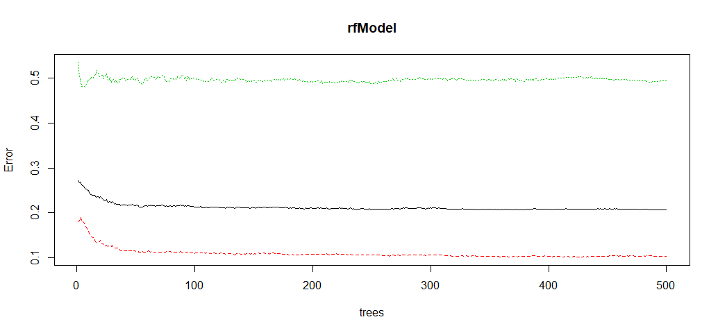
We use this plot to help us determine the number of trees. As the number of trees increases, the OOB error rate decreases, and then becomes almost constant. We are not able to decrease the OOB error rate after about 100 to 200 trees.
Tune Random Forest Model
t <- tuneRF(training[, -18], training[, 18], stepFactor = 0.5, plot = TRUE, ntreeTry = 200, trace = TRUE, improve = 0.05)
Gives this plot:
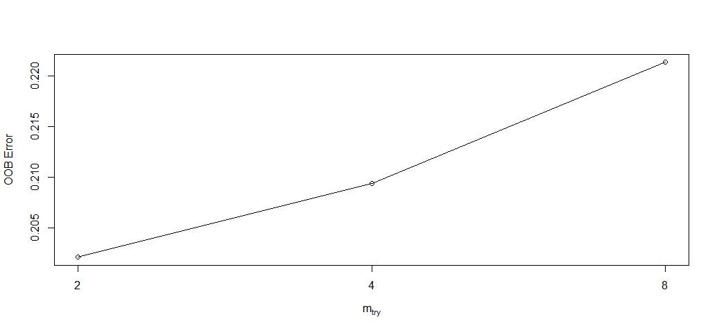
We use this plot to give us some ideas on the number of mtry to choose. OOB error rate is at the lowest when mtry is 2. Therefore, we choose mtry=2.
Fit the Random Forest Model After Tuning
rfModel_new <- randomForest(Churn ~., data = training, ntree = 200, mtry = 2, importance = TRUE, proximity = TRUE)
print(rfModel_new)
Call:
 randomForest(formula = Churn ~ ., data = training, ntree = 200,      mtry = 2, importance = TRUE, proximity = TRUE)
               Type of random forest: classification
                     Number of trees: 200
No. of variables tried at each split: 2

        OOB estimate of  error rate: 19.7%
Confusion matrix:
      No Yes class.error
No  3301 314   0.0868603
Yes  656 653   0.5011459
OOB error rate decreased to 19.7% from 20.65% earlier.
Random Forest Predictions and Confusion Matrix After Tuning
pred_rf_new <- predict(rfModel_new, testing)
caret::confusionMatrix(pred_rf_new, testing$Churn)
Confusion Matrix and Statistics

          Reference
Prediction   No  Yes
       No  1404  305
       Yes  144  255

               Accuracy : 0.787
                 95% CI : (0.7689, 0.8043)
    No Information Rate : 0.7343
    P-Value [Acc > NIR] : 1.252e-08

                  Kappa : 0.3989
 Mcnemar's Test P-Value : 4.324e-14

            Sensitivity : 0.9070
            Specificity : 0.4554
         Pos Pred Value : 0.8215
         Neg Pred Value : 0.6391
             Prevalence : 0.7343
         Detection Rate : 0.6660
   Detection Prevalence : 0.8107
      Balanced Accuracy : 0.6812

       'Positive' Class : No
The accuracy did not increase but the sensitivity improved, compare with the initial Random Forest model.
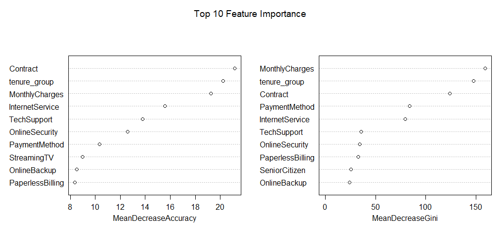
Random Forest Feature Importance
varImpPlot(rfModel_new, sort=T, n.var = 10, main = 'Top 10 Feature Importance')
Gives this plot:
Summary
From the above example, we can see that Logistic Regression and Random Forest performed better than Decision Tree for customer churn analysis for this particular dataset.
Throughout the analysis, I have learned several important things:
1. Features such as tenure_group, Contract, PaperlessBilling, MonthlyCharges and InternetService appear to play a role in customer churn.
2. There does not seem to be a relationship between gender and churn.
3. Customers in a month-to-month contract, with PaperlessBilling and are within 12 months tenure, are more likely to churn; On the other hand, customers with one or two year contract, with longer than 12 months tenure, that are not using PaperlessBilling, are less likely to churn.
Source code that created this post can be found here. I would be pleased to receive feedback or questions on any of the above.
LogModel <- glm(Churn ~ .,family=binomial(link="logit"),data=training)
print(summary(LogModel))
Every time I am running this code, this error is appearing
Error in model.frame.default(formula = training ~ ., data = training, :
invalid type (list) for variable 'training'
I got the same mistake.. Did you find any solution? I could really apreciate your help.
Check Luigi’s comment. He has re-written the code .
LogModel <- glm(as.factor(Churn) ~ ., family = binomial(link='logit'), data = training) print(summary(LogModel)) here as.factor() will transform the yes or no to binary 0 and 1.
The article is extremely helpful ma’am. I do have a query though:
You recoded the tenure column using the code:
group_tenure=0 & tenure 12 & tenure 24 & tenure 48 & tenure 60){
return(‘>60month’)
}
}
The code looks incoherent and a little blur to what you are trying to do here.
Thank you in advance!
Hi Susan, thanks for sharing your analysis. It’s a very helpful example. Did you have access to more information about the data background? For instance, to confirm the value labels of SeniorCitizen variables. I went to IBM website and didn’t find further description.
Hi Susan,
Interesting article. However, I am surprised you didn’t try to account for the fact that your data is imbalanced (especially in the RF approach). You end up having a pretty low Specificity (0.4554).
Hi Susan,
Very good article. I really enjoying it, going through the code, replicating your approach, looking at the data and trying to understand the way you drew conclusions.
I have the following questions for you:
1) Odd Ratio
There are 3 numbers there OR, 2.5%, 97.5%
1.a) what are these columns telling you?
1.b) in your github you write after the odd ratio that “For each unit increase in Monthly Charge, there is a 2.4% decrease in the likelihood of a customer’s churning”. How do you draw such a conclusion?
2) Decision Tree
2.a) Why do you focus on these variables: Contract, tenure_group, PaperlessBilling.
2.b) How did you identify these variables?
3) EDI
3.a) In which case you should eliminate a categorical variable from the analysis? Can you please give me an example in terms of percentage. When you can say that a given variable does not present enough variation and therefore you exclude from the analysis
3.b) You kept the categorical variables. Say that the dataset had 60+ variables, most of them categorical, with many levels. What is the best way to deal with this case? Generally I convert the factors into numeric, using the underlying level that R assigns. Is this a good method? There is a better method?
Luigi,
Thanks for your comments.
1 a). confint() is to calculate confidence interval for logistic regression, coef() function extracts model coefficients.
1 b). The coefficients I got gives me this suggestion.
2 a). I uses these three variables for plot only, illustration purpose. and I used all variables to fit the model.
2 b). I have explained what the plot tells us about these three variables.
3 a). I should have eliminated phone service variable.
3 b). I don’t know exactly which is the best method until I try. Mostly, I convert categorical variables to dummy variables. I just try different method every time.
Thanks
Susan
LogModel <- glm(Churn ~ .,family=binomial(link="logit"),data=training)
print(summary(LogModel))
Every time I am running this code, this error is appearing
Error in model.frame.default(formula = training ~ ., data = training, :
invalid type (list) for variable 'training'
Can you help me out, Mr. Luigi
Hi Susan,
I noticed that something is missing here:
pred_rf <- predict(rfModel, testing)
In your code the level are different, because the predictions are {"No", "Yes"} while the testset contains {0,1} therefore I needed to use ifelse to convert them at the same level.
Hi Susan,
How do you evaluate the performance of the logistic regression? Can you please check your code? In the testing you have an array of strings that are “0” or “1” while when you use the predict on the testing set you have numbers. You have this line of code that is incomplete:
fitted.results 0.5,1,0)
What are you trying to do? Are you rounding the numbers and converting them to a string so that you can compare? I think there are some bit missing.
For the above I have done the following:
fitted.results <- round(fitted.results, 0)
fitted.results <- as.character(fitted.results)
And I have an accuracy of 0.8040 (I am not sure if I had to have the same accuracy you had because we used the same seed)
I think it should read
fitted.results 0.5, 1, 0)
Thanks for the article. It is very good. I have one question about Step 3 when you group the tenure. I looked at the code and it seems that some parenthesis are missing. There is a closed curly bracket ( } ) not matched with the open, same goes with the open bracket. Are you sure it is correct?
I used the following code to do what you are trying to do there:
churn$tenure_group 60 Month”))
– sure you do not need Inf, because you checked the maximum before so you can replace the Inf with the maximum that you know from before
LogModel <- glm(Churn ~ .,family=binomial(link="logit"),data=training)
print(summary(LogModel))
Every time I am running this code, this error is appearing
Error in model.frame.default(formula = training ~ ., data = training, :
invalid type (list) for variable 'training'
can you help me here Mr. Luigi
It would help if you gave a definition of what a 1 or 0 means for the Churn variable. Does a 1 mean stopped service? It is the target variable but not explained.
If the var is called churn, I think if it is 1 there was a churn, 0 otherwise. I am not sure, this is how things should be.
This is a good basic rundown, but I’m curious why you wouldn’t include an XGBoost fit and an AUROC analysis for each fit.