Apache Spark is quickly gaining steam both in the headlines and real-world adoption, mainly because of its ability to process streaming data. With so much data being processed on a daily basis, it has become essential for us to be able to stream and analyze it in real time. In addition, Apache Spark is fast enough to perform exploratory queries without sampling. Many industry experts have provided all the reasons why you should use Spark for Machine Learning?
So, here we are now, using Spark Machine Learning Library to solve a multi-class text classification problem, in particular, PySpark.
If you would like to see an implementation in Scikit-Learn, read the previous article.
The Data
Our task is to classify San Francisco Crime Description into 33 pre-defined categories. The data can be downloaded from Kaggle.
Given a new crime description comes in, we want to assign it to one of 33 categories. The classifier makes the assumption that each new crime description is assigned to one and only one category. This is multi-class text classification problem.
-
* Input: Descript
* Example: “STOLEN AUTOMOBILE”
* Output: Category
* Example: VEHICLE THEFT
To solve this problem, we will use a variety of feature extraction technique along with different supervised machine learning algorithms in Spark. Let’s get started!
Data Ingestion and Extraction
Loading a CSV file is straightforward with Spark csv packages.
from pyspark.sql import SQLContext
from pyspark import SparkContext
sc =SparkContext()
sqlContext = SQLContext(sc)
data = sqlContext.read.format('com.databricks.spark.csv').options(header='true', inferschema='true').load('train.csv')
That’s it! We have loaded the dataset. Let’s start exploring.
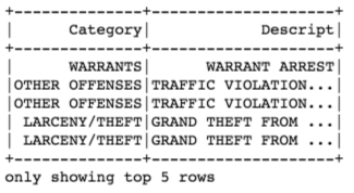
Remove the columns we do not need and have a look the first five rows:
drop_list = ['Dates', 'DayOfWeek', 'PdDistrict', 'Resolution', 'Address', 'X', 'Y']
data = data.select([column for column in data.columns if column not in drop_list])
data.show(5)
Gives this output:
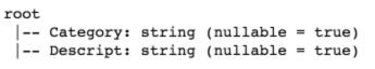
Apply printSchema() on the data which will print the schema in a tree format:
data.printSchema()
Gives this output:
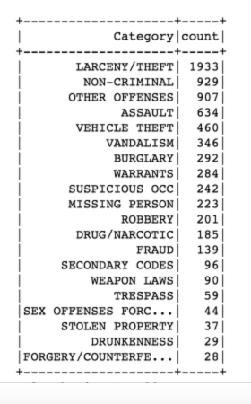
Top 20 crime categories:
from pyspark.sql.functions import col
data.groupBy("Category") \
    .count() \
    .orderBy(col("count").desc()) \
    .show()
Gives this output:
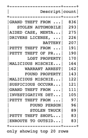
Top 20 crime descriptions:
data.groupBy("Descript") \
    .count() \
    .orderBy(col("count").desc()) \
    .show()
Gives this output:
Model Pipeline
Spark Machine Learning Pipelines API is similar to Scikit-Learn. Our pipeline includes three steps:
-
1. regexTokenizer: Tokenization (with Regular Expression)
2. stopwordsRemover: Remove Stop Words
3. countVectors: Count vectors (“document-term vectors”)
from pyspark.ml.feature import RegexTokenizer, StopWordsRemover, CountVectorizer
from pyspark.ml.classification import LogisticRegression
# regular expression tokenizer
regexTokenizer = RegexTokenizer(inputCol="Descript", outputCol="words", pattern="\\W")
# stop words
add_stopwords = ["http","https","amp","rt","t","c","the"]
stopwordsRemover = StopWordsRemover(inputCol="words", outputCol="filtered").setStopWords(add_stopwords)
# bag of words count
countVectors = CountVectorizer(inputCol="filtered", outputCol="features", vocabSize=10000, minDF=5)
StringIndexer
StringIndexer encodes a string column of labels to a column of label indices. The indices are in [0, numLabels), ordered by label frequencies, so the most frequent label gets index 0.
In our case, the label column (Category) will be encoded to label indices, from 0 to 32; the most frequent label (LARCENY/THEFT) will be indexed as 0.
from pyspark.ml import Pipeline
from pyspark.ml.feature import OneHotEncoder, StringIndexer, VectorAssembler
label_stringIdx = StringIndexer(inputCol = "Category", outputCol = "label")
pipeline = Pipeline(stages=[regexTokenizer, stopwordsRemover, countVectors, label_stringIdx])
# Fit the pipeline to training documents.
pipelineFit = pipeline.fit(data)
dataset = pipelineFit.transform(data)
dataset.show(5)
Gives this plot:
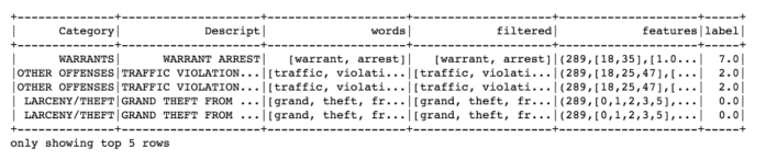
Partition Training & Test sets
# set seed for reproducibility
(trainingData, testData) = dataset.randomSplit([0.7, 0.3], seed = 100)
print("Training Dataset Count: " + str(trainingData.count()))
print("Test Dataset Count: " + str(testData.count()))
Training Dataset Count: 5185
Test Dataset Count: 2104
Model Training and Evaluation
Logistic Regression using Count Vector Features
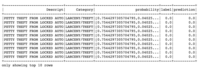
Our model will make predictions and score on the test set; we then look at the top 10 predictions from the highest probability.
lr = LogisticRegression(maxIter=20, regParam=0.3, elasticNetParam=0)
lrModel = lr.fit(trainingData)
predictions = lrModel.transform(testData)
predictions.filter(predictions['prediction'] == 0) \
    .select("Descript","Category","probability","label","prediction") \
    .orderBy("probability", ascending=False) \
    .show(n = 10, truncate = 30)
Gives this output:
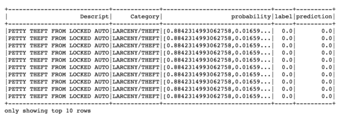
from pyspark.ml.evaluation import MulticlassClassificationEvaluator
evaluator = MulticlassClassificationEvaluator(predictionCol="prediction")
evaluator.evaluate(predictions)
0.9610787444388802
The accuracy is excellent!
Logistic Regression using TF-IDF Features
from pyspark.ml.feature import HashingTF, IDF
hashingTF = HashingTF(inputCol="filtered", outputCol="rawFeatures", numFeatures=10000)
idf = IDF(inputCol="rawFeatures", outputCol="features", minDocFreq=5) #minDocFreq: remove sparse terms
pipeline = Pipeline(stages=[regexTokenizer, stopwordsRemover, hashingTF, idf, label_stringIdx])
pipelineFit = pipeline.fit(data)
dataset = pipelineFit.transform(data)
(trainingData, testData) = dataset.randomSplit([0.7, 0.3], seed = 100)
lr = LogisticRegression(maxIter=20, regParam=0.3, elasticNetParam=0)
lrModel = lr.fit(trainingData)
predictions = lrModel.transform(testData)
predictions.filter(predictions['prediction'] == 0) \
    .select("Descript","Category","probability","label","prediction") \
    .orderBy("probability", ascending=False) \
    .show(n = 10, truncate = 30)
Gives this output:
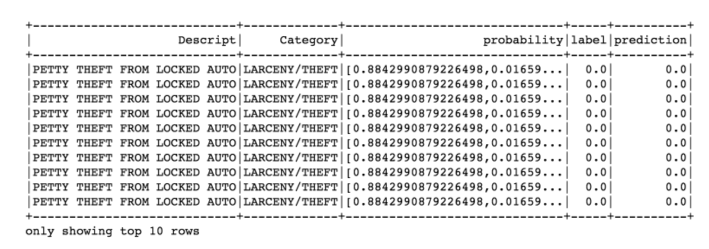
evaluator = MulticlassClassificationEvaluator(predictionCol="prediction")
evaluator.evaluate(predictions)
0.9616202660247297
The result is the same.
Cross-Validation
Let’s now try cross-validation to tune our hyper parameters, and we will only tune the count vectors Logistic Regression.
pipeline = Pipeline(stages=[regexTokenizer, stopwordsRemover, countVectors, label_stringIdx])
pipelineFit = pipeline.fit(data)
dataset = pipelineFit.transform(data)
(trainingData, testData) = dataset.randomSplit([0.7, 0.3], seed = 100)
lr = LogisticRegression(maxIter=20, regParam=0.3, elasticNetParam=0)
from pyspark.ml.tuning import ParamGridBuilder, CrossValidator
# Create ParamGrid for Cross Validation
paramGrid = (ParamGridBuilder()
             .addGrid(lr.regParam, [0.1, 0.3, 0.5]) # regularization parameter
             .addGrid(lr.elasticNetParam, [0.0, 0.1, 0.2]) # Elastic Net Parameter (Ridge = 0)
#            .addGrid(model.maxIter, [10, 20, 50]) #Number of iterations
#            .addGrid(idf.numFeatures, [10, 100, 1000]) # Number of features
             .build())
# Create 5-fold CrossValidator
cv = CrossValidator(estimator=lr, \
                    estimatorParamMaps=paramGrid, \
                    evaluator=evaluator, \
                    numFolds=5)
cvModel = cv.fit(trainingData)

predictions = cvModel.transform(testData)
# Evaluate best model
evaluator = MulticlassClassificationEvaluator(predictionCol="prediction")
evaluator.evaluate(predictions)
0.9851796929217101
The performance improved.
Naive Bayes
from pyspark.ml.classification import NaiveBayes
nb = NaiveBayes(smoothing=1)
model = nb.fit(trainingData)
predictions = model.transform(testData)
predictions.filter(predictions['prediction'] == 0) \
    .select("Descript","Category","probability","label","prediction") \
    .orderBy("probability", ascending=False) \
    .show(n = 10, truncate = 30)
Gives this output:
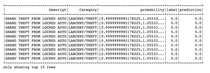
evaluator = MulticlassClassificationEvaluator(predictionCol="prediction")
evaluator.evaluate(predictions)
0.9625414629888848
Random Forest
from pyspark.ml.classification import RandomForestClassifier
rf = RandomForestClassifier(labelCol="label", \
                            featuresCol="features", \
                            numTrees = 100, \
                            maxDepth = 4, \
                            maxBins = 32)
# Train model with Training Data
rfModel = rf.fit(trainingData)
predictions = rfModel.transform(testData)
predictions.filter(predictions['prediction'] == 0) \
    .select("Descript","Category","probability","label","prediction") \
    .orderBy("probability", ascending=False) \
    .show(n = 10, truncate = 30)
Gives this output:
evaluator = MulticlassClassificationEvaluator(predictionCol="prediction")
evaluator.evaluate(predictions)
0.6600326922344301
Random forest is a very good, robust and versatile method, however it’s no mystery that for high-dimensional sparse data it’s not a best choice.
It is obvious that Logistic Regression will be our model in this experiment, with cross-validation.
This brings us to the end of the article. Source code that create this post can be found on Github.
I look forward to hearing any feedback or questions.