
I kept running into the same pattern in clustering tutorials: fit k-means, draw an elbow plot, pick a k, color the scatter, describe the segments. The validation step, when it appears at all, is a silhouette width or a bootstrap stability score, and it always seems to pass.
That bothered me, because k-means will happily partition anything. Hand it a featureless cloud of noise and it returns tidy, well-separated groups. So I wanted to answer a narrow question: can the standard validation toolkit tell the difference between data that really contains groups and data that does not? I ran the experiment, and the answer surprised me enough to write it up.
Short version: bootstrap stability, the check most often held up as the rigorous one, could not tell them apart at all.
The data
I used the Coffee Quality Institute ratings distributed through TidyTuesday: professional cuppers scoring arabica lots on aroma, flavor, aftertaste, acidity, body and balance. It is a good test case because "are there distinct coffee flavor profiles?" is a real question someone would reach for k-means to answer.
library(tidyverse)
library(cluster)
library(fpc)
library(diptest)

url <- paste0("https://raw.githubusercontent.com/rfordatascience/tidytuesday/",
              "master/data/2020/2020-07-07/coffee_ratings.csv")

coffee <- read_csv(url, show_col_types = FALSE) |>
  filter(species == "Arabica") |>
  select(aroma, flavor, aftertaste, acidity, body, balance) |>
  drop_na() |>
  filter(if_all(everything(), ~ .x > 0))   # a few lots scored all zeros

X <- scale(coffee)
dim(X)
## [1] 1310    6
That leaves 1310 coffees on 6 sensory scores. One thing to note before clustering, because it matters later:
round(cor(coffee), 2)
##            aroma flavor aftertaste acidity body balance
## aroma       1.00   0.74       0.69    0.61 0.55    0.61
## flavor      0.74   1.00       0.86    0.74 0.66    0.73
## aftertaste  0.69   0.86       1.00    0.71 0.67    0.76
## acidity     0.61   0.74       0.71    1.00 0.61    0.64
## body        0.55   0.66       0.67    0.61 1.00    0.67
## balance     0.61   0.73       0.76    0.64 0.67    1.00
pca <- prcomp(X)
round(summary(pca)$importance[2, 1:3], 3)
##   PC1   PC2   PC3
## 0.739 0.079 0.063
Every score correlates with every other score between 0.55 and 0.86, and the first principal component absorbs 73.9% of the variance with near-identical loadings on all six variables. Coffees that score well on aroma score well on everything. This looks like one general quality dimension rather than distinct profiles, but let us proceed exactly as a tutorial would and see what the diagnostics say.
The standard pipeline
dsp_colors <- c("#0066CC", "#E8862D", "#159A6C", "#7D5BD6",
                "#D64580", "#2AA9B8", "#C9A227")
dsp_theme <- theme_minimal(base_size = 13) +
  theme(plot.background    = element_rect(fill = "#ECECEF", color = NA),
        panel.background   = element_rect(fill = "#ECECEF", color = NA),
        panel.grid.minor   = element_blank(),
        panel.grid.major.x = element_blank(),
        panel.grid.major.y = element_line(color = "grey78"),
        axis.ticks         = element_blank(),
        plot.title         = element_text(face = "bold"),
        strip.text         = element_text(face = "bold"))

elbow <- map_dfr(1:10, ~ tibble(
  k   = .x,
  wss = kmeans(X, .x, nstart = 25, iter.max = 50)$tot.withinss
))

ggplot(elbow, aes(k, wss)) +
  geom_line(color = dsp_colors[1], linewidth = 0.9) +
  geom_point(color = dsp_colors[1], size = 2.4) +
  scale_x_continuous(breaks = 1:10) +
  labs(title = "The elbow says three",
       x = "Number of clusters (k)",
       y = "Total within-cluster sum of squares") +
  dsp_theme
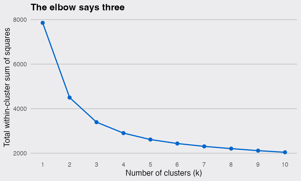
A textbook elbow at k = 3. The drop in within-cluster sum of squares is 3,354 going from one cluster to two, 1,107 going to three, then only 490 going to four. So k = 3 it is.
km3 <- kmeans(X, 3, nstart = 25, iter.max = 50)

coffee |>
  mutate(cluster = km3$cluster) |>
  group_by(cluster) |>
  summarise(n = n(), across(everything(), ~ round(mean(.x), 2))) |>
  arrange(flavor)
## # A tibble: 3 × 8
##   cluster     n aroma flavor aftertaste acidity  body balance
##     <int> <dbl> <dbl>  <dbl>      <dbl>   <dbl> <dbl>   <dbl>
## 1       2   298  7.23   7.09       6.97    7.19  7.22    7.1
## 2       1   706  7.58   7.54       7.42    7.53  7.52    7.54
## 3       3   306  7.88   7.89       7.79    7.9   7.83    7.89
Three clean groups. But look at the summary rows: the clusters are ordered on every single variable at once. Cluster means rise together across aroma, flavor, aftertaste, acidity, body and balance. These are not flavor profiles, they are quality tiers, which is what you get when you cut a one-dimensional gradient into three pieces. The cluster means on PC1 confirm it:
round(tapply(pca$x[, 1], km3$cluster, mean), 2)
##     1     2     3
## -0.06  2.82 -2.61
The three checks, and how they do
Now the validation. I ran the three diagnostics that show up most often.
Silhouette width measures how much closer each point sits to its own cluster than to the next nearest one, averaged over all points. Kaufman and Rousseeuw’s rule of thumb is that below 0.25 there is no substantial structure, and 0.25 to 0.50 is weak.
sil_k <- function(M, k) {
  km <- kmeans(M, k, nstart = 25, iter.max = 50)
  mean(silhouette(km$cluster, dist(M))[, 3])
}
coffee_sil <- sil_k(X, 3)
round(coffee_sil, 3)
## [1] 0.303
The gap statistic compares the within-cluster dispersion to what you would get on a structureless reference distribution, and cluster::clusGap picks a k for you.
gap_coffee <- clusGap(X, FUN = kmeans, nstart = 25, K.max = 8, B = 50)
maxSE(gap_coffee$Tab[, "gap"], gap_coffee$Tab[, "SE.sim"], method = "firstSEmax")
## [1] 3
round(gap_coffee$Tab[, "gap"], 3)
## [1] 1.138 1.200 1.248 1.250 1.251 1.245 1.235 1.223
Bootstrap stability is the one usually presented as the serious check. fpc::clusterboot resamples the data, re-clusters, matches the new clusters to the original ones and reports a mean Jaccard similarity per cluster. Above 0.85 is conventionally called highly stable.
jac_k <- function(M, k, seed) {
  cb <- clusterboot(M, B = 100, clustermethod = kmeansCBI, krange = k,
                    runs = 25, count = FALSE, seed = seed)
  mean(cb$bootmean)
}
coffee_jac <- jac_k(X, 3, seed = 7)
round(coffee_jac, 3)
## [1] 0.963
So: silhouette 0.303 (weak, but tutorials publish worse), gap statistic endorsing k = 3, and a bootstrap Jaccard of 0.963, comfortably in "highly stable" territory. Two of the three checks pass, and the one that is lukewarm would not stop most people.
The control
Here is the part I actually wanted to run. I generated a dataset with the same number of rows, the same number of variables and the same covariance matrix as the coffee scores, drawn from a single multivariate normal. By construction it contains zero clusters. Then I put it through the identical pipeline.
null_like <- function(M) {
  N <- MASS::mvrnorm(nrow(M), mu = rep(0, ncol(M)), Sigma = cov(M))
  colnames(N) <- colnames(M)
  N
}
X_null <- null_like(X)
project <- function(M, label) {
  pc <- prcomp(M)$x
  tibble(PC1 = pc[, 1], PC2 = pc[, 2], data = label,
         cluster = factor(kmeans(M, 3, nstart = 25, iter.max = 50)$cluster))
}

bind_rows(project(X, "Coffee scores (real data)"),
          project(X_null, "Random data, no clusters at all")) |>
  ggplot(aes(PC1, PC2, color = cluster)) +
  geom_point(alpha = 0.55, size = 1.2) +
  facet_wrap(~ data) +
  scale_color_manual(values = dsp_colors) +
  labs(title = "Same pipeline, same picture", x = "PC1", y = "PC2") +
  dsp_theme +
  theme(legend.position = "none")
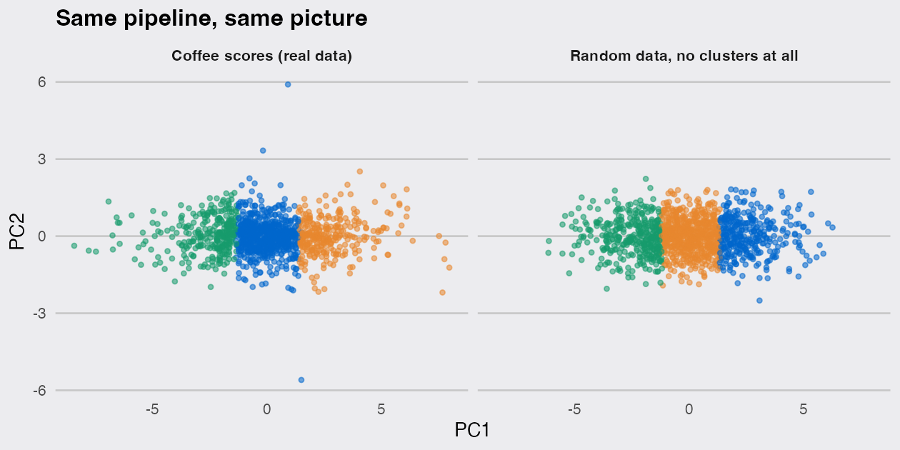
Both panels show three crisp, well-separated, roughly equal bands. The right panel is pure noise. Nothing in that picture distinguishes the real data from the fake, because in both cases k-means is doing the same thing: slicing a single elongated blob into three along its longest axis.
The diagnostics on the noise:
c(silhouette = round(sil_k(X_null, 3), 3),
  jaccard    = round(jac_k(X_null, 3, seed = 7), 3))
## silhouette    jaccard
##      0.273      0.925
A structureless cloud scores about as well as the coffee data on silhouette and just as well on bootstrap stability.
Calibrating against the null
One draw could be luck, so I repeated it. Twenty null datasets, each matched to the real data’s size and covariance, each pushed through the same two checks. I did the same for a positive control: the palmerpenguins body measurements, where three real species are known to be present.
penguins_X <- palmerpenguins::penguins |>
  drop_na(bill_length_mm, bill_depth_mm, flipper_length_mm, body_mass_g) |>
  select(bill_length_mm, bill_depth_mm, flipper_length_mm, body_mass_g) |>
  scale()

calibrate <- function(M, k, R = 20) {
  map_dfr(1:R, function(i) {
    N <- null_like(M)
    tibble(rep = i, silhouette = sil_k(N, k), jaccard = jac_k(N, k, seed = i))
  })
}

null_coffee   <- calibrate(X, 3)
null_penguins <- calibrate(penguins_X, 3)

observed <- tibble(
  data       = c("Coffee", "Penguins"),
  silhouette = c(coffee_sil, sil_k(penguins_X, 3)),
  jaccard    = c(coffee_jac, jac_k(penguins_X, 3, seed = 7))
)
observed |> mutate(across(where(is.numeric), ~ round(.x, 3)))
## # A tibble: 2 × 3
##   data     silhouette jaccard
##   <chr>         <dbl>   <dbl>
## 1 Coffee        0.303   0.963
## 2 Penguins      0.447   0.965
nulls <- bind_rows(mutate(null_coffee, data = "Coffee"),
                   mutate(null_penguins, data = "Penguins")) |>
  pivot_longer(c(silhouette, jaccard), names_to = "index", values_to = "null")

obs_long <- observed |>
  pivot_longer(c(silhouette, jaccard), names_to = "index", values_to = "obs")

labels <- c(silhouette = "Silhouette width", jaccard = "Bootstrap Jaccard")

ggplot(nulls, aes(y = data)) +
  geom_point(aes(x = null), color = "grey55", alpha = 0.6, size = 1.8) +
  geom_point(data = obs_long, aes(x = obs), color = dsp_colors[2], size = 4) +
  facet_wrap(~ index, scales = "free_x", labeller = labeller(index = labels)) +
  labs(title = "Observed value (orange) against 20 null datasets (grey)",
       x = NULL, y = NULL) +
  dsp_theme +
  theme(panel.grid.major.y = element_blank(),
        panel.grid.major.x = element_line(color = "grey78"))
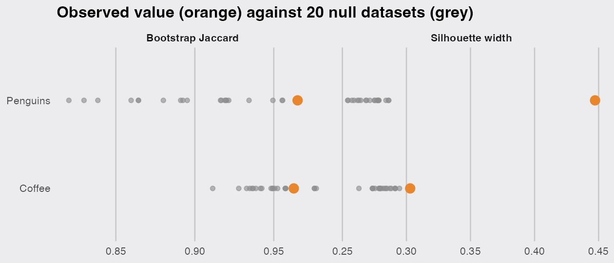
This is the result worth taking away. On bootstrap Jaccard, the orange dots are buried in the grey. The coffee continuum scores 0.963, squarely inside its own null range of 0.911 to 0.977. The penguins, which genuinely contain three species, score 0.965 against a null range of 0.82 to 0.956, clearing the noise by 0.009. Real groups, an artificial cut through a gradient, and pure noise all land in the same narrow band above 0.9, and the ordering between them is meaningless.
That is not a bug in clusterboot. It is what the statistic measures. Jaccard stability asks whether the algorithm reproduces the same partition on resampled data, and a smooth elongated cloud has extremely reproducible cut points, precisely because there is nothing there to make the boundary wobble. High stability is evidence that your k-means run is deterministic, not that your clusters exist.
Silhouette does better, but only once it is calibrated. Raw, the coffee value of 0.303 and the penguin value of 0.447 are both "weak" by the usual thresholds. Against their own nulls the picture separates: coffee clears its null range (0.263 to 0.295) by only 0.008, while the penguins beat their null range (0.254 to 0.286) by 0.161, a margin roughly 19 times larger. The absolute number was uninformative. The comparison was informative.
A note on the gap statistic, which I left out of that plot because it behaves differently:
gap_k <- function(M) {
  g <- clusGap(M, FUN = kmeans, nstart = 25, K.max = 8, B = 50)
  maxSE(g$Tab[, "gap"], g$Tab[, "SE.sim"], method = "firstSEmax")
}
c(noise = gap_k(X_null), coffee = gap_k(X), penguins = gap_k(penguins_X))
##    noise   coffee penguins
##        1        3        5
Run on the pure noise it correctly returns k = 1, so it is not useless. But it endorsed k = 3 on the coffee continuum, and on the penguins it misses the three species. Its reference distribution is a uniform box, so it responds to any departure from uniformity, skewness included, and not to clustering specifically.
What did work
If the question is "are there groups", then a better thing to test is whether the data is multimodal along the direction that carries the structure. Hartigan and Hartigan’s dip test does exactly that, and diptest::dip.test is one line.
dip_coffee   <- dip.test(prcomp(X)$x[, 1])
dip_penguins <- dip.test(prcomp(penguins_X)$x[, 1])
c(coffee = dip_coffee$p.value, penguins = dip_penguins$p.value)
##       coffee     penguins
## 8.544241e-01 2.465773e-05
bind_rows(
  tibble(pc1 = scale(prcomp(X)$x[, 1])[, 1],
         data = "Coffee: one bump"),
  tibble(pc1 = scale(prcomp(penguins_X)$x[, 1])[, 1],
         data = "Penguins: two bumps")
) |>
  ggplot(aes(pc1)) +
  geom_density(fill = dsp_colors[1], color = NA, alpha = 0.75) +
  facet_wrap(~ data, scales = "free_y") +
  labs(title = "The check that separated them",
       x = "First principal component (scaled)", y = "Density") +
  dsp_theme
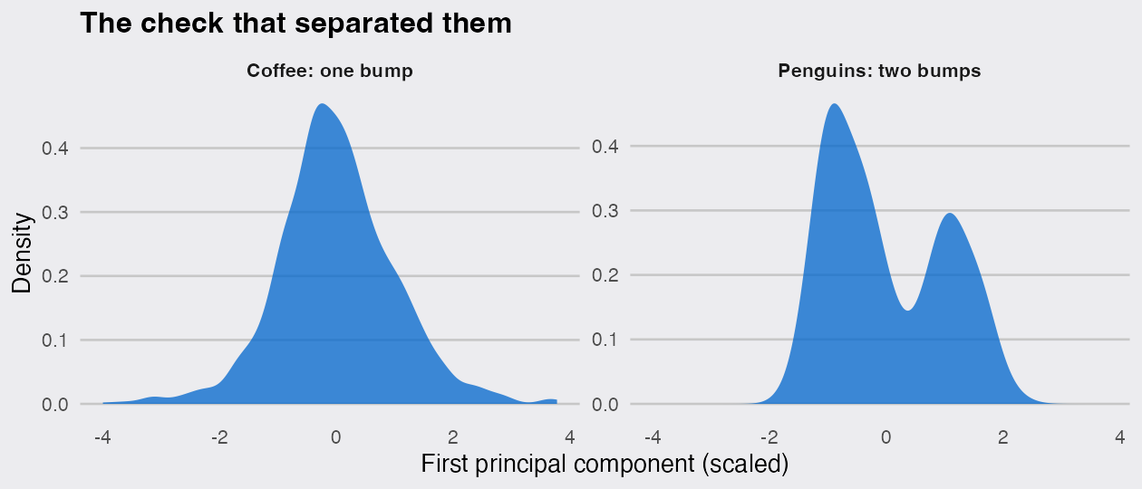
The coffee scores give p = 0.85, entirely consistent with a single bump. The penguins give p = 2.5e-05. That is the separation the other two indices failed to make, from a test that took a fraction of a second.
The honest caveat: the dip test here looks only at PC1. Groups could separate along some other direction and this would miss them, so on a real problem run it on the first few components, or on the pairwise distance distribution.
What I would do instead
Three things came out of this that I will apply from now on.
Always run a matched null. null_like() above is four lines. Generate data with your data’s covariance and no clusters, run your entire pipeline on it, and report your index next to that reference. Any index without a null is a number without a scale, and as this showed, the thresholds people quote from memory can be met by noise.
Do not treat stability as evidence of existence. Bootstrap Jaccard is a genuinely useful statistic for a different question: given that groups exist, which of my clusters are solid and which are an artifact of a few points. Reported as proof that the groups are real, it will agree with you no matter what.
Set runs when you call clusterboot. kmeansCBI defaults to runs = 1, a single random start per bootstrap replicate. On the penguins that default made the Jaccard swing between roughly 0.63 and 0.86 depending only on the seed, because k-means kept landing in local optima. With runs = 25 it is stable across seeds. If you have ever seen a stability score change when you changed the seed, this is likely why.
And when the data really is a continuum, as the coffee scores are, cutting it into three is still a perfectly reasonable thing to do. Quality tiers are useful. Just describe them as what they are, thresholds on a gradient that you chose, rather than as types you discovered. The difference matters to whoever reads the result next and assumes the groups were out there waiting.


