
The variable importance plot is the part of a random forest most people actually read. The model itself is a few hundred trees nobody will inspect, so the ranking of predictors is what ends up in the summary, the slide, and the conclusion. I wanted to know how much weight that ranking can carry, so I handed a forest four columns I knew in advance were meaningless and looked at where it put them.
One of them came second.
library(tidyverse)
library(randomForest)
library(ranger)
I am using Chicago’s Energy Benchmarking data, which large buildings in the city are required to report every year. The outcome is site energy use intensity (EUI, in kBtu per square foot), and the predictors are the things you would reach for first: what kind of building it is, where it is, how big it is, how old it is, and how many buildings the record covers.
url <- paste0("https://data.cityofchicago.org/resource/xq83-jr8c.csv?",
              "data_year=2023&$limit=5000")

bldg <- read_csv(url, show_col_types = FALSE) |>
  filter(reporting_status == "Submitted", !is.na(site_eui_kbtu_sq_ft)) |>
  transmute(
    site_eui       = site_eui_kbtu_sq_ft,
    property_type  = fct_lump_min(factor(str_squish(primary_property_type)), 20),
    community_area = fct_lump_min(factor(str_squish(community_area)), 10),
    floor_area     = gross_floor_area_buildings_sq_ft,
    year_built     = year_built,
    n_buildings    = of_buildings
  ) |>
  drop_na()

glimpse(bldg)
## Rows: 2,583
## Columns: 6
## $ site_eui       <dbl> 87.8, 34.8, 57.8, 155.1, 83.8, 81.8, 91.7, 54.9, 63.1, …
## $ property_type  <fct> Multifamily Housing, Office, Multifamily Housing, Other…
## $ community_area <fct> Kenwood, Near North Side, Near North Side, Hyde Park, N…
## $ floor_area     <dbl> 59310, 632163, 258647, 5252, 177380, 627680, 63979, 919…
## $ year_built     <dbl> 1950, 1991, 2007, 1926, 1948, 1974, 1957, 1980, 1927, 1…
## $ n_buildings    <dbl> 1, 1, 1, 1, 6, 1, 3, 1, 1, 1, 1, 1, 1, 1, 1, 1, 1, 1, 1…
That leaves 2583 buildings, with 12 property types and 49 community areas. Both factors are pooled with fct_lump_min() for a reason I come back to below: randomForest() refuses any categorical predictor with more than 53 categories, and Chicago has 77 community areas.
Now the four columns that carry no information at all. Each is drawn independently of the buildings and of each other, so the honest importance of every one of them is zero. They differ only in how many distinct values they take: a coin flip, a 10-level factor, a 50-level factor, and a continuous uniform draw.
set.seed(2026)
n <- nrow(bldg)

dat <- bldg |>
  mutate(
    noise_coin   = factor(sample(c("heads", "tails"), n, replace = TRUE)),
    noise_cat10  = factor(sample(1:10, n, replace = TRUE)),
    noise_cat50  = factor(sample(1:50, n, replace = TRUE)),
    noise_number = runif(n)
  )
Why does my random forest rank a random column as important?
Because the importance measure you get by default is impurity-based, and impurity importance rewards a predictor for having many distinct values, not for being predictive. A variable with 50 categories gives the split search 50 groups to shuffle into two piles, and with that many candidate splits it will find one that separates the outcome by luck alone. The forest then credits it for the separation.
Here is the same forest scored both ways.
set.seed(1)
fit <- randomForest(site_eui ~ ., data = dat, importance = TRUE, ntree = 500)

imp <- randomForest::importance(fit) |>
  as_tibble(rownames = "variable") |>
  rename(perm = `%IncMSE`, impurity = IncNodePurity) |>
  mutate(distinct_values = map_int(variable, ~ n_distinct(dat[[.x]])),
         rank_impurity   = rank(-impurity),
         rank_perm       = rank(-perm)) |>
  arrange(rank_impurity)

imp
## # A tibble: 9 × 6
##   variable         perm impurity distinct_values rank_impurity rank_perm
##   <chr>           <dbl>    <dbl>           <int>         <dbl>     <dbl>
## 1 property_type  30.8   1912837.              12             1         1
## 2 noise_cat50    -2.56  1351743.              50             2         8
## 3 community_area  6.89   975308.              49             3         2
## 4 noise_cat10    -1.22   444888.              10             4         7
## 5 year_built      1.49   408452.             145             5         5
## 6 floor_area      5.55   405809.            2345             6         3
## 7 noise_number   -2.95   303707.            2583             7         9
## 8 n_buildings     3.42    68712.              23             8         4
## 9 noise_coin     -0.592   41951.               2             9         6
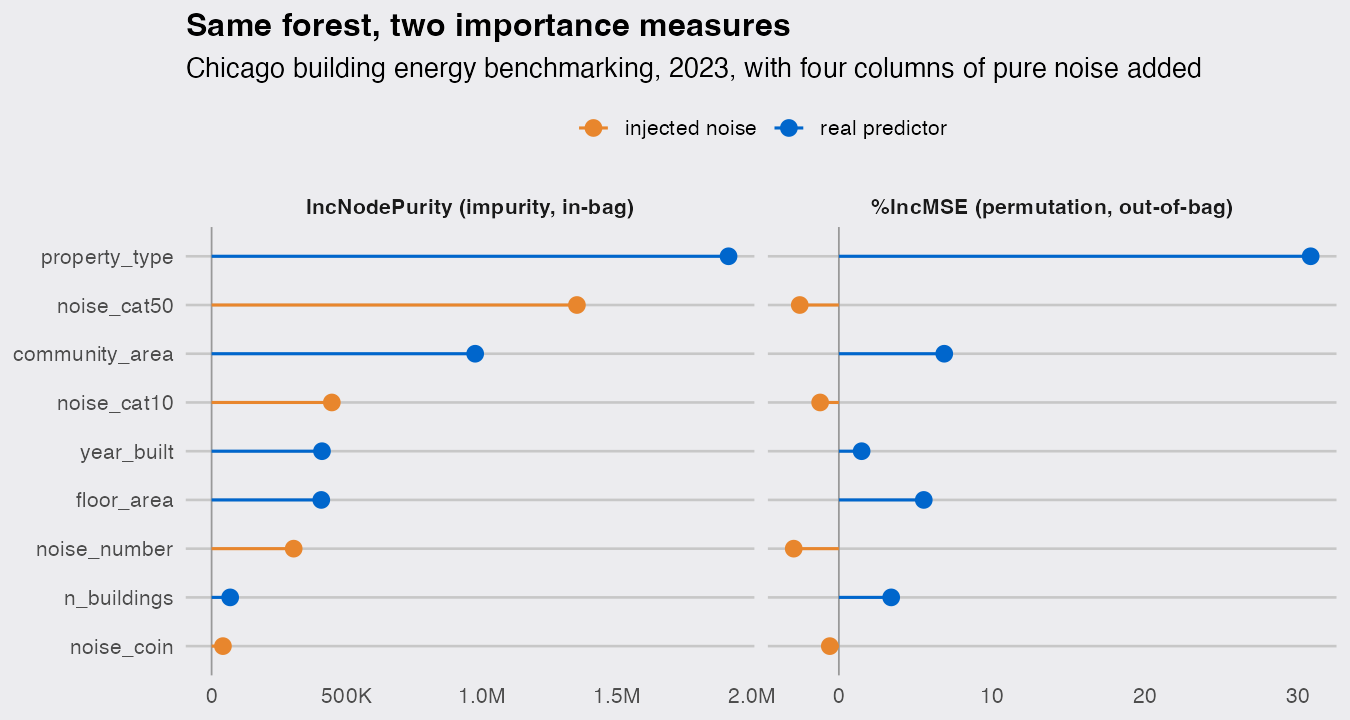
noise_cat50 is the second most important variable in the building, ahead of floor area, age, and location. It outranks 4 of the 5 real predictors on its own; noise_cat10, in fourth place, outranks 3. Read down the perm column instead and the picture inverts completely: all four noise columns come out negative, and the five real predictors take the top five places.
This is not a fluke of one seed. Regenerating both the noise and the forest across eight seeds, noise_cat50 came second on impurity every single time and noise_cat10 came fourth every single time.
What is the difference between IncNodePurity and %IncMSE?
IncNodePurity is the total drop in node impurity (residual sum of squares, for a regression forest) summed over every split that used that variable, measured on the rows that were in the tree. %IncMSE is permutation importance: for each tree, the out-of-bag rows are scored, the variable is shuffled, they are scored again, and the loss of accuracy is recorded.
The difference that matters is which rows each one uses. Impurity is computed on the same data the split was chosen to fit, so a variable that can carve those rows finely is credited for doing so, whether or not the carving generalises. Permutation importance is computed out of bag, on rows the tree never saw, where a lucky split has nothing left to be lucky about.
There is a trap in how you get them. randomForest() has importance = FALSE by default, and with the default call importance(fit) returns a single column, IncNodePurity. You have to opt in to the measure that is not biased:
set.seed(1)
default_fit <- randomForest(site_eui ~ ., data = dat, ntree = 200)
colnames(randomForest::importance(default_fit))
## [1] "IncNodePurity"
colnames(randomForest::importance(fit))
## [1] "%IncMSE"       "IncNodePurity"
So the ranking that a plain randomForest() call plus varImpPlot() puts in front of you is the impurity one. For a regression forest I would read %IncMSE with scale = FALSE, which returns the raw increase in mean squared error rather than dividing by its standard error. On this data all four noise columns come out negative that way, which is the answer you want from a variable that means nothing.
round(randomForest::importance(fit, type = 1, scale = FALSE), 2)
##                %IncMSE
## property_type   952.91
## community_area  148.89
## floor_area       99.67
## year_built       25.19
## n_buildings       8.18
## noise_coin       -3.06
## noise_cat10     -20.67
## noise_cat50     -56.38
## noise_number    -27.25
A version you can run on built-in data
Nothing here depends on Chicago. This block uses quakes, which ships with R, and reproduces the whole effect in six lines. As of randomForest 4.7-1.2 on R 4.6.1:
library(randomForest)

set.seed(1)
q <- quakes
q$junk <- factor(sample(1:50, nrow(q), replace = TRUE))   # pure noise

fq <- randomForest(mag ~ ., data = q, importance = TRUE)
round(randomForest::importance(fq, scale = FALSE), 3)
##          %IncMSE IncNodePurity
## lat        0.010        13.341
## long       0.015        15.914
## depth      0.014        17.665
## stations   0.144        81.481
## junk      -0.001        26.563
junk ranks second of five on IncNodePurity, above latitude, longitude and depth, while its permutation importance is essentially zero. The only real predictor of earthquake magnitude in that table, the number of stations that reported the event, wins on both measures, but three genuine variables lose to a random draw on the impurity ranking.
Does the bias grow with the number of levels?
It grows steeply, and it is close to a straight function of how many distinct values the column has. I refit the same forest six times over, each time with a single pure-noise factor added, varying only its level count, five forests per setting.
set.seed(11)

sweep <- expand_grid(k = c(2, 5, 10, 20, 35, 50), rep = 1:5) |>
  pmap(function(k, rep) {
    d <- bldg |> mutate(noise = factor(sample(seq_len(k), n, replace = TRUE)))
    f <- randomForest(site_eui ~ ., data = d, ntree = 200)
    tibble(k = k, rep = rep,
           impurity = randomForest::importance(f)["noise", "IncNodePurity"])
  }) |>
  list_rbind()

sweep |> group_by(k) |> summarise(mean_impurity = mean(impurity))
## # A tibble: 6 × 2
##       k mean_impurity
##   <dbl>         <dbl>
## 1     2       120822.
## 2     5       342683.
## 3    10       615582.
## 4    20       961081.
## 5    35      1246470.
## 6    50      1448523.
set.seed(99)
ref_fit <- randomForest(site_eui ~ ., data = bldg, ntree = 200)
ref <- randomForest::importance(ref_fit) |>
  as_tibble(rownames = "variable") |>
  rename(value = IncNodePurity)
ref
## # A tibble: 5 × 2
##   variable          value
##   <chr>             <dbl>
## 1 property_type  1810583.
## 2 community_area  835869.
## 3 floor_area      671986.
## 4 year_built      601833.
## 5 n_buildings     138842.
A meaningless binary column earns about 121,000 in impurity. The same column with 50 levels earns 1,449,000, a factor of 12, and that puts it above every real predictor in this dataset except property type. The crossings are the useful part of the figure: pure noise passes building age at around 10 levels, floor area just after, and community area at around 20.
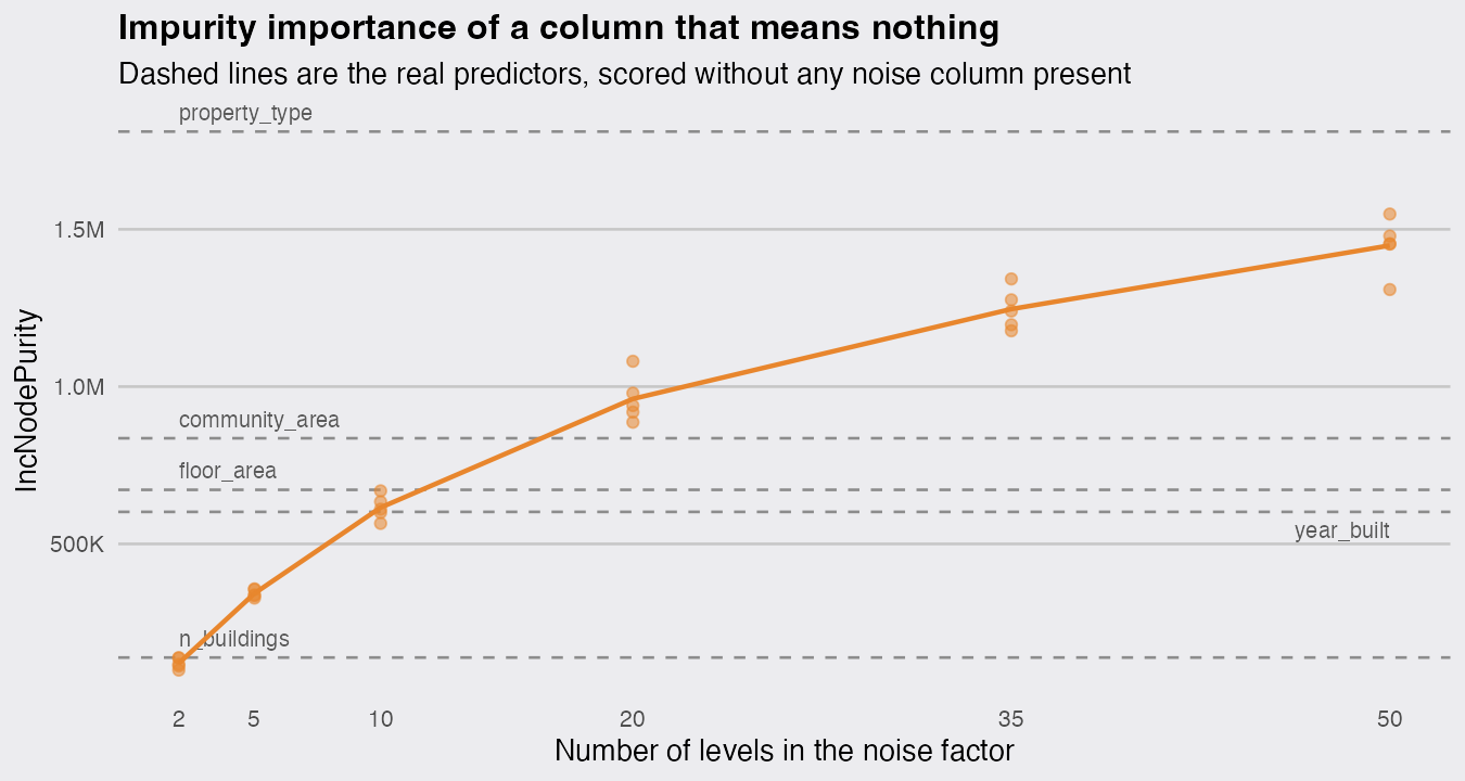
Continuous noise lands in the same regime rather than off the scale. The noise_number column has 2583 distinct values but scores like a factor with somewhere between 10 and 20 levels, because a numeric split search only considers cut points along one fixed ordering, while a factor with k levels can be partitioned far more freely. Free-text identifiers, ZIP codes, model numbers and product SKUs are the columns to watch for: high cardinality, low information, and they will float to the top of an impurity ranking.
How do I get unbiased variable importance in R?
Ask for permutation importance explicitly. In randomForest that is importance = TRUE at fit time and type = 1 when you read it. In ranger, which fits the same forest a good deal faster, it is one argument:
set.seed(7)
rg <- ranger(site_eui ~ ., data = dat, num.trees = 1000,
             importance = "permutation", respect.unordered.factors = "order")

sort(rg$variable.importance, decreasing = TRUE) |> round(1)
##  property_type     floor_area community_area     year_built    n_buildings
##         1420.9          182.9          166.1          136.1           16.8
##    noise_cat50    noise_cat10     noise_coin   noise_number
##            6.5            3.5           -9.2          -16.3
Every real predictor beats every noise column, including n_buildings, which is the weakest genuine variable here.
The respect.unordered.factors argument is worth setting deliberately. ranger 0.18.0 defaults to "ignore", which treats an unordered factor as though its levels already came in a meaningful order, and on this data the default costs the real factor and rewards the fake one:
set.seed(7)
rg_default <- ranger(site_eui ~ ., data = dat, num.trees = 1000,
                     importance = "permutation")

sort(rg_default$variable.importance, decreasing = TRUE) |> round(1)
##  property_type     floor_area     year_built community_area    noise_cat50
##         1603.1          220.8          122.0          104.8           91.6
##    n_buildings     noise_coin    noise_cat10   noise_number
##           22.3           -6.3          -17.1          -30.0
community_area falls from 166.1 to 104.8, while noise_cat50 climbs from 6.5 to 91.6 and lands just behind it. Permutation importance is unbiased about cardinality either way, but it can only measure what the splitting rule was able to use.
ranger also offers importance = "impurity_corrected", the actual impurity reduction of Nembrini, König and Wright (2018), which subtracts the impurity a permuted copy of the variable would have earned and comes with importance_pvalues(). It is a genuine fix for the cardinality bias, but it is not a drop-in one when unordered factors are in play. ranger warns that corrected impurity "may not be unbiased for re-ordered factor levels", and it means it:
set.seed(7)
rg_air <- ranger(site_eui ~ ., data = dat, num.trees = 1000,
                 importance = "impurity_corrected",
                 respect.unordered.factors = "order")

sort(rg_air$variable.importance, decreasing = TRUE) |> round()
##  property_type community_area    noise_cat50     floor_area     year_built
##        1523719         268497         166113         108941         104660
##    n_buildings     noise_coin   noise_number    noise_cat10
##          19503           1387         -38681         -55848
noise_cat50 comes third of nine, still above floor area and building age. Switching to "ignore" removes the warning but brings back the problem from the previous block. When the predictors include unordered factors with many levels, which is exactly the case where the bias bites hardest, permutation importance is the measure I trust without extra care.
What the junk columns cost the model
Misranking is not the only damage. The four noise columns also make the forest measurably worse, because mtry samples three of nine variables at each split, and a split that lands on a 50-level random factor is a split spent on nothing.
set.seed(1); with_noise    <- randomForest(site_eui ~ ., data = dat,  ntree = 500)
set.seed(1); without_noise <- randomForest(site_eui ~ ., data = bldg, ntree = 500)

c(with_noise    = 100 * tail(with_noise$rsq, 1),
  without_noise = 100 * tail(without_noise$rsq, 1)) |> round(1)
##    with_noise without_noise
##          26.6          35.3
Out-of-bag variance explained goes from 35.3 percent to 26.6 percent, a loss of 8.8 points, from adding columns that contain nothing. Random forests are often described as robust to irrelevant predictors, and they are, in the sense that they do not break. They are not free of them.
What I would take away
Fit with importance = TRUE and read the permutation column, in either package. If a high-cardinality identifier ranks near the top of an impurity plot, check it against permutation importance before writing a sentence about it. And treat the 53-level limit in randomForest() as a hint rather than an obstacle: the factors it refuses to accept are the ones most likely to fool the default measure if you pool them just enough to squeeze them in.
The Chicago result that survives all of this is unremarkable and worth stating plainly, because it is the one the biased ranking obscured: what a building is for explains far more of its energy intensity than where it is, how big it is, or how old it is. Property type carries about 7.8 times the permutation importance of the next variable, and the ordering underneath it only becomes readable once the noise is scored honestly.

