
Playing at home is worth about half what it was in international football. In the 1980s a national team playing at home scored 55% more goals than it would have against the same opponent on neutral ground. In the matches played since 2020 it scores 25% more. I expected the raw home records to show the same decline, and they don’t: home teams outscored their visitors by between 1.60 and 1.72 goals to 1 in every decade since the 1970s, and by 1.64 to 1 since 2020.
The two measures part ways because of who visits whom. In 1980s friendlies the host was, on average, the weaker of the two teams; in friendlies since 2020 it is clearly the stronger one, so more of the raw home record is strong teams beating weak guests. Between two evenly matched teams, the host’s chance of winning has fallen from 55% to 46%.
The match data
Mart Jürisoo’s international football results dataset (CC0) lists men’s full internationals since 1872: 49,945 matches up to 6 October 2026, with both scores, the tournament, and a neutral flag that is TRUE when the match was played at a neutral venue. A host nation’s own matches at a tournament it hosts are not neutral. Home advantage can only be measured off neutral ground, so a match counts as a home match for the first-listed team only when neutral is FALSE.
How do I estimate home advantage in R?
Fit a Poisson regression of goals on a home indicator, with one fixed effect for the scoring team and one for its opponent, and exponentiate the home coefficient: it is the factor by which playing at home multiplies a team’s goals against the same opponent. The team and opponent effects stand for each side’s attack and defence, so the home effect is measured net of who was playing whom. This is the model from Maher (1982). The block below runs on its own with readr 2.2.0, dplyr 1.2.1 and fixest 0.14.2 on R 4.6.1, and fits the matches since 2020:
library(tidyverse)
library(fixest)

matches <- read_csv(
  "https://raw.githubusercontent.com/martj42/international_results/master/results.csv",
  show_col_types = FALSE
) |>
  filter(!is.na(home_score)) |>   # scheduled fixtures have no score yet
  mutate(id = row_number())

# One row per team per match. The first-listed team is only at home off neutral ground.
long <- bind_rows(
  matches |> transmute(id, date, tournament, neutral, team = home_team, opp = away_team,
                       goals = home_score, home = !neutral),
  matches |> transmute(id, date, tournament, neutral, team = away_team, opp = home_team,
                       goals = away_score, home = FALSE)
)

# Two rows per match, so cluster the standard errors on the match
recent <- fepois(goals ~ home | team + opp, data = filter(long, year(date) >= 2020),
                 vcov = ~id)
recent
## Poisson estimation, Dep. Var.: goals
## Observations: 13,058
## Fixed-effects: team: 256,  opp: 256
## Standard-errors: Clustered (id)
##          Estimate Std. Error z value  Pr(>|z|)
## homeTRUE 0.225177   0.016379 13.7477 < 2.2e-16 ***
## ---
## Signif. codes:  0 '***' 0.001 '**' 0.01 '*' 0.05 '.' 0.1 ' ' 1
## Log-Likelihood: -17,707.8   Adj. Pseudo R2: 0.14023
##            BIC:  40,267.9     Squared Cor.: 0.399193
exp(coef(recent))
## homeTRUE
## 1.252544
The home coefficient is 0.23, and its exponential, 1.25, says a team at home scores 25% more than it would against the same opponent at a neutral venue. glm(goals ~ home + team + opp, family = poisson) fits the same model and returns the same number, but it estimates 532 coefficients to get there and took 22 seconds here, against a fraction of a second for fepois(), which absorbs the team effects instead of estimating them as dummy columns.
Home records stayed flat while the home edge halved
Fitting the model separately in each five-year window lets every team’s strength change over time while the home effect is estimated afresh. The raw ratio next to it is total home goals over total away goals in the same non-neutral matches.
fit_home <- function(d) {
  m <- fepois(goals ~ home | team + opp, data = d, vcov = ~id, notes = FALSE)
  off_neutral <- filter(d, !neutral)
  tibble(venue = exp(coef(m)[["homeTRUE"]]),
         lo    = exp(confint(m)["homeTRUE", 1]),
         hi    = exp(confint(m)["homeTRUE", 2]),
         raw   = sum(off_neutral$goals[off_neutral$home]) / sum(off_neutral$goals[!off_neutral$home]),
         n     = n_distinct(d$id),
         mid   = mean(decimal_date(d$date)))   # plot each window at its average match date
}

windows <- long |>
  filter(year(date) >= 1960) |>
  mutate(start = 5 * (year(date) %/% 5)) |>
  nest(.by = start) |>
  mutate(fit = map(data, fit_home)) |>
  select(start, fit) |>
  unnest(fit) |>
  arrange(start)
dsp_colors <- c("#0066CC", "#E8862D", "#159A6C", "#7D5BD6",
                "#D64580", "#2AA9B8", "#C9A227")
dsp_theme <- theme_minimal(base_size = 13) +
  theme(plot.background    = element_rect(fill = "#ECECEF", color = NA),
        panel.background   = element_rect(fill = "#ECECEF", color = NA),
        panel.grid.minor   = element_blank(),
        panel.grid.major.x = element_blank(),
        panel.grid.major.y = element_line(color = "grey78"),
        axis.ticks         = element_blank(),
        plot.title         = element_text(face = "bold"),
        strip.text         = element_text(face = "bold"))

plot_data <- windows |>
  pivot_longer(c(raw, venue), names_to = "measure") |>
  mutate(lo = if_else(measure == "raw", NA, lo),
         hi = if_else(measure == "raw", NA, hi),
         measure = if_else(measure == "raw", "Raw: home goals per away goal",
                           "Model: home effect against the same opponent"))

ggplot(plot_data, aes(mid, value, color = measure, fill = measure)) +
  geom_hline(yintercept = 1, color = "grey45") +
  geom_ribbon(aes(ymin = lo, ymax = hi), alpha = 0.2, color = NA, show.legend = FALSE) +
  geom_line(linewidth = 1.1) +
  geom_point(size = 2) +
  scale_color_manual(values = dsp_colors[c(2, 1)]) +
  scale_fill_manual(values = dsp_colors[c(2, 1)]) +
  scale_x_continuous(breaks = seq(1960, 2030, 10)) +
  scale_y_continuous(limits = c(1, NA), labels = \(x) paste0(x, "x")) +
  labs(x = NULL, y = NULL,
       title = "Home teams still outscore visitors. The venue explains less of it",
       subtitle = "Men's internationals off neutral ground, five-year windows (2025-26 so far)",
       color = NULL, fill = NULL) +
  dsp_theme +
  theme(legend.position = "top", legend.justification = "left")
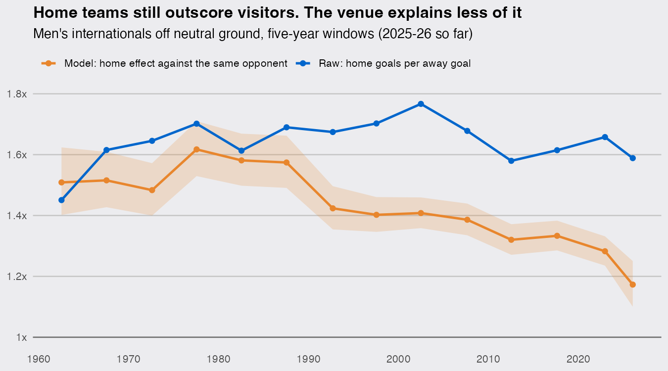
The home effect peaked at 1.62 in 1975-79 and was 1.28 in 2020-24. The first 1,803 matches of 2025-26 give 1.17. Over the same windows since 1970 the raw ratio never left the range 1.58 to 1.77. The decline is not a pandemic artifact either: the matches since 2022 alone give 1.26, and the slide started in the early 1990s.
Why the raw ratio misses it: who hosts whom
A raw home ratio mixes two things, what the venue does and how much stronger the host is than its visitor, and the model can separate them. Predicting every non-neutral match with home set to FALSE leaves only the two teams’ strengths, so the ratio of those predictions says how much more the host would score at a neutral venue. Here it is per decade, for friendlies and competitive matches separately:
strength_edge <- function(d) {
  m <- fepois(goals ~ home | team + opp, data = d, vcov = ~id, notes = FALSE)
  d |>
    mutate(neutral_pred = predict(m, newdata = mutate(d, home = FALSE))) |>
    filter(!neutral) |>
    summarise(venue    = exp(coef(m)[["homeTRUE"]]),
              strength = sum(neutral_pred[home], na.rm = TRUE) / sum(neutral_pred[!home], na.rm = TRUE),
              raw      = sum(goals[home]) / sum(goals[!home]))
}

by_decade <- long |>
  filter(year(date) >= 1960) |>
  mutate(decade = 10 * (year(date) %/% 10), friendly = tournament == "Friendly")

decades_all <- by_decade |>
  nest(.by = decade) |>
  mutate(fit = map(data, strength_edge)) |>
  select(decade, fit) |>
  unnest(fit)

by_type <- by_decade |>
  nest(.by = c(decade, friendly)) |>
  mutate(fit = map(data, strength_edge)) |>
  select(decade, friendly, fit) |>
  unnest(fit) |>
  arrange(friendly, decade)

by_type
## # A tibble: 14 × 5
##    decade friendly venue strength   raw
##     <dbl> <lgl>    <dbl>    <dbl> <dbl>
##  1   1960 FALSE     1.51    1.04   1.81
##  2   1970 FALSE     1.50    1.10   1.99
##  3   1980 FALSE     1.56    1.02   1.93
##  4   1990 FALSE     1.40    1.08   1.79
##  5   2000 FALSE     1.40    1.14   1.84
##  6   2010 FALSE     1.36    1.06   1.58
##  7   2020 FALSE     1.25    1.12   1.53
##  8   1960 TRUE      1.47    0.887  1.34
##  9   1970 TRUE      1.62    0.844  1.39
## 10   1980 TRUE      1.56    0.867  1.38
## 11   1990 TRUE      1.46    1.03   1.54
## 12   2000 TRUE      1.37    1.08   1.55
## 13   2010 TRUE      1.34    1.13   1.64
## 14   2020 TRUE      1.24    1.53   2.05
In competitive matches, where qualifying groups play home and away, the host’s strength edge stays between 1.02 and 1.14 in every decade, and the raw ratio falls with the home effect, from 1.93 in the 1980s to 1.53 since 2020. Friendlies are where the hosts changed. In 1980s friendlies the host was expected to score 0.87 goals for each one its visitor scored at a neutral venue; since 2020 it is 1.53. So the raw home ratio in friendlies rose from 1.38 to 2.05 while the home effect in the same matches fell from 1.56 to 1.24. Any comparison of home records across eras, or across teams that schedule different friendlies, has the same problem.
What the drop is worth in a match
Take two evenly matched teams that each score 1.36 goals a match at a neutral venue, the average since 2020, and let the host’s rate carry the home effect of each era:
mu <- mean(filter(long, year(date) >= 2020)$goals)

result_probs <- function(home_effect, mu) {
  p <- outer(dpois(0:20, mu * home_effect), dpois(0:20, mu))   # rows: host goals
  tibble(win = sum(p[lower.tri(p)]), draw = sum(diag(p)), loss = sum(p[upper.tri(p)]))
}

odds <- tibble(era = c("neutral", "1980s", "2020s"),
               home_effect = c(1, decades_all$venue[decades_all$decade == 1980],
                               decades_all$venue[decades_all$decade == 2020])) |>
  mutate(probs = map(home_effect, result_probs, mu = mu)) |>
  unnest(probs)

odds
## # A tibble: 3 × 5
##   era     home_effect   win  draw  loss
##   <chr>         <dbl> <dbl> <dbl> <dbl>
## 1 neutral        1    0.372 0.257 0.372
## 2 1980s          1.55 0.547 0.209 0.244
## 3 2020s          1.25 0.457 0.236 0.307
At a neutral venue each side wins 37% of the time. With the 1980s home effect the host wins 55% and loses 24%; with the effect since 2020 it wins 46% and loses 31%. This data cannot say why the venue matters less, and the usual explanations would need data it does not have. What it does say is where not to look: the raw home record of national teams has barely moved in fifty years, because the venue’s shrinking share has been filled by who gets invited.

