When you need to run a logistic regression in R, your modeling routine is probably three base functions: glm() to fit, predict() to score, and broom’s tidy() to turn the fit into a table of odds ratios. Meanwhile tidymodels keeps showing up, and it can replace every one of those functions. The fair questions are: what actually changes when you swap them, what does the rest of the framework add that base R does not, and does any of it earn a place in epidemiological research?
Let’s answer all three on real data. First I replace glm(), predict(), and tidy() with their tidymodels equivalents one for one and see what is different (mostly the output, not the math). Then I show what tidymodels adds around the model, the part base R has no direct function for. Finally I weigh whether it is worth using for everyday epidemiological research.
The data: predicting diabetes in NHANES
I use NHANES ↗, the US National Health and Nutrition Examination Survey, which ships as an R package. NHANES is a complex survey with sampling weights, and any valid population estimate has to carry those weights (using the survey ↗ package and survey::svyglm() in place of glm()). For this tutorial, I keep the example simple and unweighted.
library(tidymodels)
library(NHANES)
tidymodels_prefer() # solves naming conflicts in R by making tidymodels functions take priority over other packages
data(NHANES)
nh <- NHANES |>
  filter(Age >= 18) |>
  select(
    Diabetes,
    Age,
    BMI,
    Gender,
    PhysActive,
    BPSysAve,
    TotChol,
    DirectChol,
    Poverty,
    Smoke100
  ) |>
  filter(!is.na(Diabetes)) |>
  mutate(Diabetes = factor(Diabetes, levels = c("No", "Yes"))) |>
  distinct() # NHANES resampled some individuals; drop exact duplicate rows

head(nh)
## # A tibble: 6 × 10
##   Diabetes   Age   BMI Gender PhysActive BPSysAve TotChol DirectChol Poverty Smoke100
##   <fct>    <int> <dbl> <fct>  <fct>         <int>   <dbl>      <dbl>   <dbl> <fct>
## 1 No          34  32.2 male   No              113    3.49       1.29    1.36 Yes
## 2 No          49  30.6 female No              112    6.7        1.16    1.91 Yes
## 3 No          45  27.2 female Yes             118    5.82       2.12    5    No
## 4 No          66  23.7 male   Yes             111    4.99       0.67    2.2  Yes
## 5 No          58  23.7 male   Yes             104    4.24       0.96    5    No
## 6 No          54  26.0 male   Yes             134    6.41       1.16    2.2  No
That leaves 4,834 distinct adults, 11.3% with diagnosed diabetes. The distinct() matters more than it looks: the NHANES package is a teaching sample that resampled some individuals, so the raw extract carries many exact duplicate rows. Leave them in and copies of one person would land on both sides of the train/test split I make later, quietly flattering any out-of-sample estimate, so I keep one row per person.
Note the factor(..., levels = c("No", "Yes")): it is not cosmetic. glm() models the probability of the last level, so with No first I am modeling P(diabetes), which is what I want. Reverse it and every odds ratio silently inverts.
Replacing the base functions, one for one
glm() and broom, and their parsnip equivalent
Here is the base-R fit, tidied into odds ratios.
fit_glm <- glm(
  Diabetes ~ Age +
    BMI +
    Gender +
    PhysActive +
    BPSysAve +
    TotChol +
    DirectChol +
    Poverty +
    Smoke100,
  data = nh,
  family = binomial
)

tidy(fit_glm, exponentiate = TRUE, conf.int = TRUE) |>
  select(term, OR = estimate, conf.low, conf.high, p.value)
## # A tibble: 10 × 5
##    term               OR conf.low conf.high  p.value
##    <chr>           <dbl>    <dbl>     <dbl>    <dbl>
##  1 (Intercept)   0.00218 0.000670   0.00693 7.77e-25
##  2 Age           1.06    1.05       1.06    1.85e-46
##  3 BMI           1.08    1.06       1.09    7.43e-22
##  4 Gendermale    1.14    0.901      1.45    2.68e- 1
##  5 PhysActiveYes 0.965   0.766      1.22    7.61e- 1
##  6 BPSysAve      1.01    1.00       1.02    2.52e- 3
##  7 TotChol       0.780   0.700      0.868   6.34e- 6
##  8 DirectChol    0.531   0.376      0.743   2.70e- 4
##  9 Poverty       0.880   0.820      0.945   4.26e- 4
## 10 Smoke100Yes   1.21    0.975      1.51    8.32e- 2
Now the same model through parsnip, the tidymodels interface: pick a model type, set an engine, fit().
fit_psn <- logistic_reg() |>
  set_engine("glm") |>
  fit(
    Diabetes ~ Age +
      BMI +
      Gender +
      PhysActive +
      BPSysAve +
      TotChol +
      DirectChol +
      Poverty +
      Smoke100,
    data = nh
  )

tidy(fit_psn, exponentiate = TRUE, conf.int = TRUE) |>
  select(term, OR = estimate, conf.low, conf.high, p.value)
## # A tibble: 10 × 5
##    term               OR conf.low conf.high  p.value
##    <chr>           <dbl>    <dbl>     <dbl>    <dbl>
##  1 (Intercept)   0.00218 0.000670   0.00693 7.77e-25
##  2 Age           1.06    1.05       1.06    1.85e-46
##  3 BMI           1.08    1.06       1.09    7.43e-22
##  4 Gendermale    1.14    0.901      1.45    2.68e- 1
##  5 PhysActiveYes 0.965   0.766      1.22    7.61e- 1
##  6 BPSysAve      1.01    1.00       1.02    2.52e- 3
##  7 TotChol       0.780   0.700      0.868   6.34e- 6
##  8 DirectChol    0.531   0.376      0.743   2.70e- 4
##  9 Poverty       0.880   0.820      0.945   4.26e- 4
## 10 Smoke100Yes   1.21    0.975      1.51    8.32e- 2
Identical coefficients, because parsnip called glm() for you and tidy() is the same broom. So far tidymodels has changed nothing.
predict(): the one replacement that actually behaves differently
Prediction is where the swap is not cosmetic. Let’s score three people with each.
newpeople <- nh[c(10, 200, 900), ]
newpeople
## # A tibble: 3 × 10
##   Diabetes   Age   BMI Gender PhysActive BPSysAve TotChol DirectChol Poverty Smoke100
##   <fct>    <int> <dbl> <fct>  <fct>         <int>   <dbl>      <dbl>   <dbl> <fct>
## 1 No          60  25.8 male   No              152    6.39       1.34    1.03 Yes
## 2 No          22  52.1 male   No              128    3.67       0.88    0.98 No
## 3 No          45  22.0 female No              114    4.78       1.55    2.03 No
# you must remember type = "response" to get a probability
predict(fit_glm, newpeople, type = "response")
##          1          2          3
## 0.14843669 0.21032214 0.03234337
With type = "response", predict() returns the three people as probabilities between 0 and 1, the modeled diabetes risk for each. Omit the argument and you get log-odds instead, which is the default trap the comment warns about.
# TIDYMODELS: always a tibble, one row per input row, standardized names
predict(fit_psn, newpeople, type = "prob") # .pred_No / .pred_Yes
## # A tibble: 3 × 2
##   .pred_No .pred_Yes
##      <dbl>     <dbl>
## 1    0.852    0.148
## 2    0.790    0.210
## 3    0.968    0.0323
tidymodels returns the same risks, but as a tibble with one column per outcome level: .pred_No and .pred_Yes, which sum to 1 in each row. There is no scale to remember, type = "prob" always means probabilities, and the column names say which level each one belongs to. .pred_Yes is the diabetes risk, the same number the type = "response" vector gave above.
augment() goes one step further and binds the predictions onto the data:
augment(fit_psn, newpeople) |>
  select(Diabetes, Age, BMI, .pred_class, .pred_Yes)
## # A tibble: 3 × 5
##   Diabetes   Age   BMI .pred_class .pred_Yes
##   <fct>    <int> <dbl> <fct>           <dbl>
## 1 No          60  25.8 No             0.148
## 2 No          22  52.1 No             0.210
## 3 No          45  22.0 No             0.0323
So the whole base-R workflow has a direct translation:
| What you want | Base R | tidymodels |
|---|---|---|
| Fit a logistic model | glm(y ~ ., family = binomial) |
logistic_reg() |> set_engine("glm") |> fit(y ~ ., data) |
| Coefficients as odds ratios | broom::tidy(fit, exponentiate = TRUE) |
tidy(fit, exponentiate = TRUE) (same broom) |
| Predicted probabilities | predict(fit, new, type = "response") (vector) |
predict(fit, new, type = "prob") (tibble) |
| Data plus predictions | cbind(new, p) |
augment(fit, new) |
Conclusion: for a single fit, tidymodels computes exactly what glm(), predict(), and broom already give you. The output is tidier and the prediction defaults are safer, but the math is the same, so the swap on its own is not a reason to switch.
What tidymodels adds
The framework is not really about replacing glm(); it is about the workflow around the model.
Preprocessing that travels with predict()
In base R, if you scale or impute your predictors, you have to redo that transformation, identically, on every new dataset you predict on, using the training statistics. Forget to, or use the new data’s own mean instead, and you get wrong or leaky predictions. A recipe attaches the preprocessing to the model so predict() applies it automatically.
set.seed(2026)
split <- initial_split(nh, prop = 0.75, strata = Diabetes)
train <- training(split)
test <- testing(split)

rec <- recipe(Diabetes ~ ., data = train) |>
  step_impute_median(all_numeric_predictors()) |> # learn medians on train
  step_impute_mode(all_nominal_predictors()) |>
  step_dummy(all_nominal_predictors()) |>
  step_normalize(all_numeric_predictors()) # center/scale on train stats

wf_fit <- workflow() |>
  add_recipe(rec) |>
  add_model(logistic_reg() |> set_engine("glm")) |>
  fit(train)
The payoff shows up when a new row is incomplete. Here is a test patient whose BMI is missing:
patient <- test[1, ]
patient$BMI <- NA_real_

# base glm cannot score a row with a gap
predict(fit_glm, patient, type = "response")
##  1
## NA
# the workflow imputes BMI (with the training median) before predicting
predict(wf_fit, patient, type = "prob")
## # A tibble: 1 × 2
##   .pred_No .pred_Yes
##      <dbl>     <dbl>
## 1    0.945    0.0551
The base model returns NA; the workflow silently imputes the missing BMI with the median it learned from the training data and returns a real risk.
Model performance
The question a risk model has to answer is how it does on data it has never seen, measured the way risk models are judged: discrimination (ROC AUC) and calibration. Fitting was the easy part; the work is estimating those two honestly, on data the fit did not touch. That is the piece base R leaves you to assemble, and where tidymodels earns its keep.
vfold_cv() splits the training data into 10 folds; the model is fit on 9 of them and scored on the tenth, ten times over, so every performance number comes from data the fit never saw. Doing this by hand means writing the fold loop and re-learning the recipe inside each fold, so the imputation and scaling use only that fold’s training portion. Get that last part wrong (impute once on the whole set) and the held-out fold has quietly seen the training data through a shared median.
set.seed(2026)
folds <- vfold_cv(train, v = 10, strata = Diabetes)

log_spec <- logistic_reg() |> set_engine("glm")
mset <- metric_set(roc_auc, brier_class) # discrimination + calibration

res_log <- fit_resamples(
  workflow() |> add_recipe(rec) |> add_model(log_spec),
  folds,
  metrics = mset
)
fit_resamples() fits the workflow on every fold, re-learns the recipe inside each one, and collects the two metrics without ever touching the test set.
collect_metrics(res_log) |>
  select(.metric, cv_estimate = mean, std_err)
## # A tibble: 2 × 3
##   .metric     cv_estimate std_err
##   <chr>             <dbl>   <dbl>
## 1 brier_class      0.0860 0.00172
## 2 roc_auc          0.816  0.0105
Cross-validated, the logistic model reaches an AUC of 0.816, and the number is trustworthy precisely because no fold was scored on data it trained on. You could get the same value in base R, but you would own the whole fold loop and the per-fold preprocessing described above. tidymodels does that bookkeeping for you: the recipe travels into every resample automatically, so the shortcut that leaks is not even on the table.
Discrimination and calibration plots
lf_log <- last_fit(
  workflow() |> add_recipe(rec) |> add_model(log_spec),
  split,
  metrics = mset
)
preds <- collect_predictions(lf_log)
dsp_colors <- c(
  "#0066CC",
  "#E8862D",
  "#159A6C",
  "#7D5BD6",
  "#D64580",
  "#2AA9B8",
  "#C9A227"
)
dsp_theme <- theme_minimal(base_size = 13) +
  theme(
    plot.background = element_rect(fill = "#ECECEF", color = NA),
    panel.background = element_rect(fill = "#ECECEF", color = NA),
    panel.grid.minor = element_blank(),
    panel.grid.major = element_line(color = "grey78"),
    axis.ticks = element_blank(),
    plot.title = element_text(face = "bold"),
    strip.text = element_text(face = "bold")
  )
preds |>
  roc_curve(truth = Diabetes, .pred_Yes, event_level = "second") |>
  ggplot(aes(1 - specificity, sensitivity)) +
  geom_abline(linetype = "dashed", color = "grey60") +
  geom_path(linewidth = 1.1, color = dsp_colors[1]) +
  coord_equal() +
  labs(
    title = "Discrimination: who is at risk of diabetes?",
    subtitle = "ROC curve on held-out test data",
    x = "False positive rate",
    y = "True positive rate"
  ) +
  dsp_theme
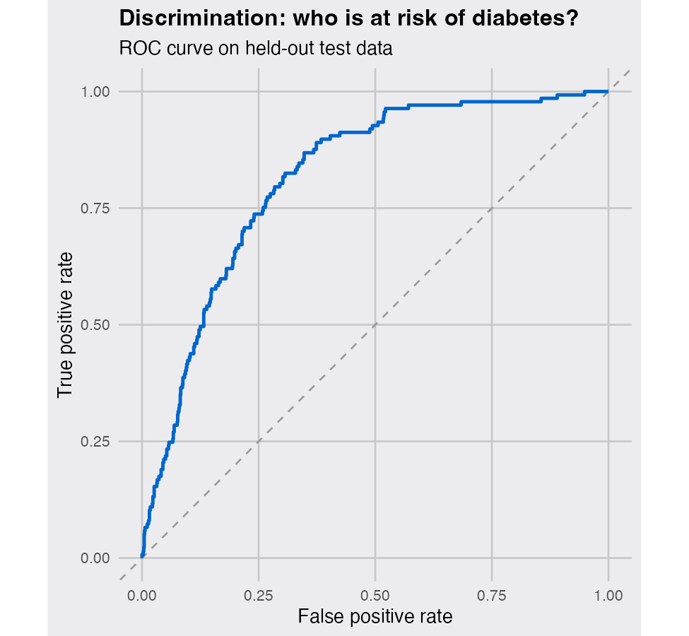
On the held-out test set the model’s AUC is 0.816, close to the cross-validated estimate, which is the reassurance you want: it did not fall apart on data it had never seen. But discrimination is only half the story. A risk model also has to be calibrated: when it predicts a 30% risk, close to 30% of the people carrying that prediction should actually have diabetes. The next plot checks that by binning people into risk deciles and comparing predicted against observed rates.
preds |>
  mutate(bin = ntile(.pred_Yes, 10)) |>
  group_by(bin) |>
  summarise(
    pred = mean(.pred_Yes),
    obs = mean(Diabetes == "Yes"),
    .groups = "drop"
  ) |>
  ggplot(aes(pred, obs)) +
  geom_abline(linetype = "dashed", color = "grey60") +
  geom_line(linewidth = 0.9, color = dsp_colors[1]) +
  geom_point(size = 2.4, color = dsp_colors[1]) +
  labs(
    title = "Calibration: are the predicted risks honest?",
    subtitle = "Predicted vs observed rate by risk decile (dashed line = perfect)",
    x = "Mean predicted risk",
    y = "Observed diabetes rate"
  ) +
  dsp_theme
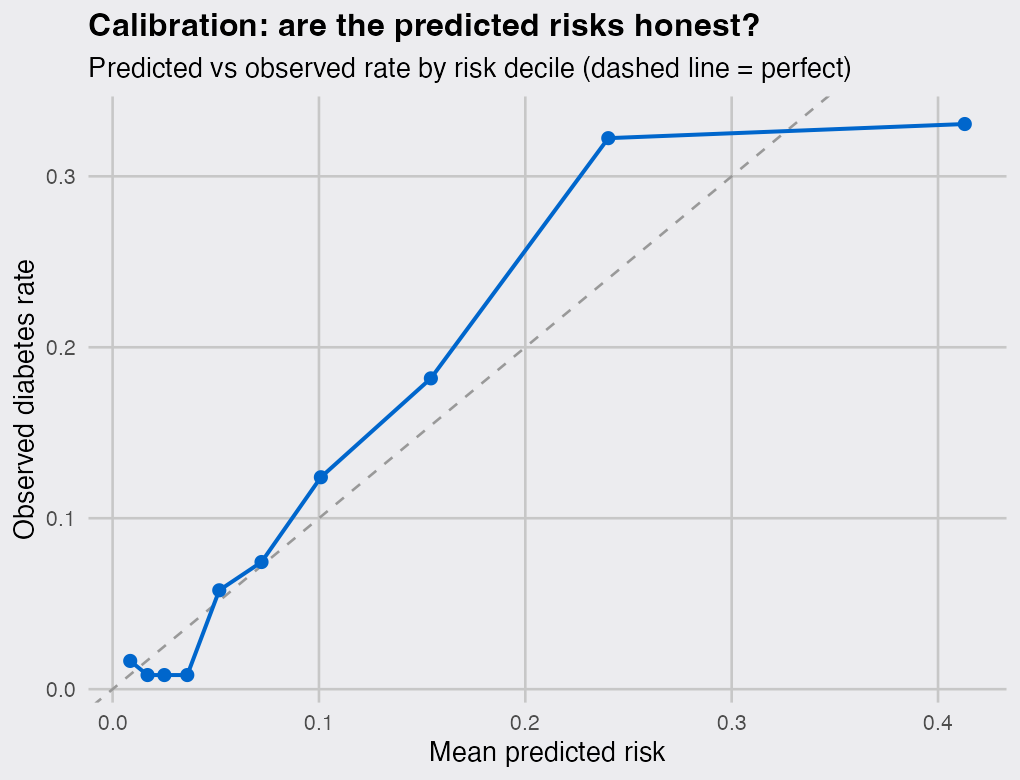
The points track the diagonal closely through the low and middle deciles and wobble only at the high-risk end, where the bins are smallest and noisiest and predicted risk climbs toward 40%. The Brier score, 0.087 (lower is better), is a single number that folds discrimination and calibration together.
Is any of this useful in epidemiological and clinical research?
It depends on the aim:
Association and etiologic papers report adjusted odds or hazard ratios with confidence intervals, usually from a survey-weighted or matched design. For that, base glm() or survey::svyglm() with broom::tidy() is exactly right and tidymodels adds almost nothing.
Prediction and prognostic papers are the other case: developing or validating a clinical risk score, the kind of work that reporting guidelines like TRIPOD govern. There the deliverable is discrimination and calibration on unseen data, with internal validation by resampling. That is what tidymodels streamlines.
So it is not glm() versus tidymodels, and broom lives inside both. Replace your base functions with tidymodels when you want the workflow it enables, not for the sake of the swap: use glm() or svyglm() and broom to explain associations, and reach for the full framework when your focus is a risk model you have to validate.
That’s it. I hope you find this tutorial useful, and if you have questions, leave a comment below.


