The biggest tenth of US counties have 17 times more physicians’ offices per resident than the smallest tenth, and only 31% as many religious organisations. A scaling exponent is the single number that summarises comparisons like that, and the usual way to get one in R is a log-log regression. Fit it to grocery stores across all 3,142 counties and it comes back at 0.80, meaning fewer stores per person as counties get bigger. The raw totals say the opposite. The gap is the 941 counties with no grocery store at all, and you cannot take the log of zero.
How do I fit a scaling exponent in R?
Regress the log of the count on the log of population and read the slope. An exponent of 1 means the count is proportional to population, above 1 means more per person in bigger places, below 1 means fewer. This block runs on its own with R 4.6.1, dplyr 1.2.1 and readr 2.2.0, on two keyless Census files.
library(dplyr)
library(readr)

zip <- tempfile(fileext = ".zip")
download.file("https://www2.census.gov/programs-surveys/cbp/datasets/2023/cbp23co.zip",
              zip, quiet = TRUE)
cbp <- read_csv(unzip(zip, "cbp23co.txt", exdir = tempdir()),
                col_select = c(fipstate, fipscty, naics, est),
                col_types = cols(.default = col_character(), est = col_integer())) |>
  mutate(fips = paste0(fipstate, fipscty))

pop <- read_csv(paste0("https://www2.census.gov/programs-surveys/popest/datasets/",
                       "2020-2024/counties/totals/co-est2024-alldata.csv"),
                col_types = cols(.default = col_character(),
                                 POPESTIMATE2023 = col_double())) |>
  filter(SUMLEV == "050") |>
  transmute(fips = paste0(STATE, COUNTY), county = CTYNAME, pop = POPESTIMATE2023) |>
  filter(fips %in% cbp$fips[cbp$naics == "------"])

grocery <- cbp |>
  filter(naics == "445110") |>                       # supermarkets and grocery stores
  select(fips, est) |>
  right_join(pop, by = "fips") |>
  mutate(est = coalesce(est, 0L))                    # no row in CBP means no store

coef(lm(log(est) ~ log(pop), data = filter(grocery, est > 0)))
## (Intercept)    log(pop)
##  -6.4439886   0.8041279
County Business Patterns counts establishments with paid employees, one row per county and industry, and a county appears under an industry only when it has at least one. The zeros are absences from the file rather than values in it, which is what the coalesce() step is for. An exponent of 0.80 says that doubling a county’s population multiplies its grocery stores by 2 to the power 0.80, or 1.75, so the number of stores per person falls 13% with every doubling.
What does R do with the counties that have none?
It refuses to fit. log(0) is -Inf, and lm() stops with NA/NaN/Inf in 'y', which is the one honest moment in this procedure. The two usual repairs are to keep only the counties with at least one establishment, or to add a small constant before taking logs, and both change the exponent.
Dropping the zeros throws away 941 of the 3,142 counties, and they are not a random 30%: the median population of a county with no grocery store is 8,025 against 44,099 for the rest. What survives at the small end of the fit are the small counties that happen to have a store, so the line is lifted on the left and flattened. Adding a constant keeps everyone but picks the answer: log(est + 1) gives 0.83 and log(est + 0.5) gives 0.96, a swing of 0.13 from a constant nobody can justify.
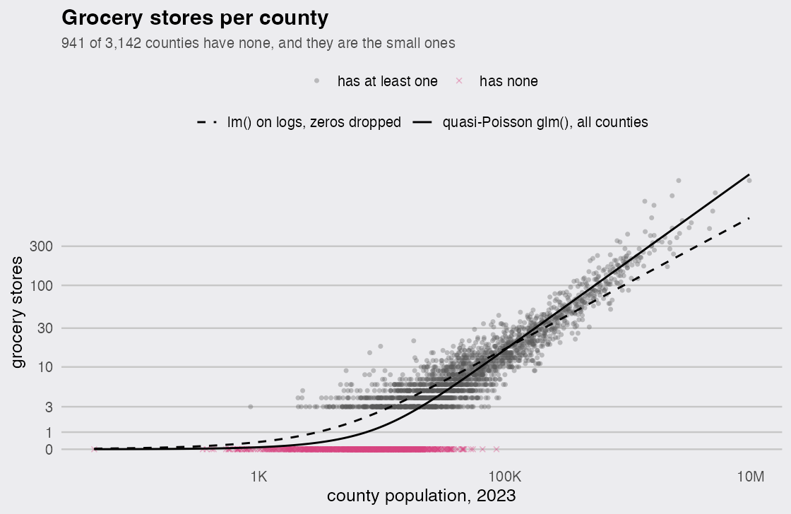
Should I use Poisson regression instead of logging the counts?
Yes. Put the log on the expected count rather than on the data, with glm(est ~ log(pop), family = quasipoisson). The log link means the coefficient on log(pop) is still the scaling exponent, zero counts are ordinary observations, and nothing has to be invented for them.
mq <- glm(est ~ log(pop), family = quasipoisson, data = grocery)
coef(mq)[2]
## log(pop)
## 1.077407
For grocery stores that is 1.08 (95% interval 1.06 to 1.09), slightly above proportional, against 0.80 from the log-log fit. A negative binomial fit, MASS::glm.nb(), puts it at 1.03, so the choice of count model moves the number far less than the choice to take logs did. Use quasipoisson rather than poisson here: the dispersion is 6.6, so plain Poisson standard errors would be about 2.6 times too small.
Simple arithmetic settles which answer is right, with no model at all. Add up the stores and the people in the smallest tenth of counties and you get 1.33 grocery stores per 10,000 residents; do the same for the largest tenth and you get 1.97. More per person in the big counties, not fewer, and the exponent implied by those two totals is 1.07.
Which businesses actually scale with county size?
Professional services concentrate, everyday infrastructure spreads out, and restaurants track people almost exactly. Physicians’ offices run 0.40 per 10,000 residents in the smallest tenth of counties and 6.87 in the largest, and dentists go from 0.15 to 4.62. Religious organisations run the other way, 14.2 per 10,000 in the smallest counties against 4.4 in the largest, and gas stations from 4.5 to 2.2. Full-service restaurants barely move: 7.9 per 10,000 in the smallest decile and 8.0 in the largest, one restaurant for every 1,250 people or so at both ends of the range.
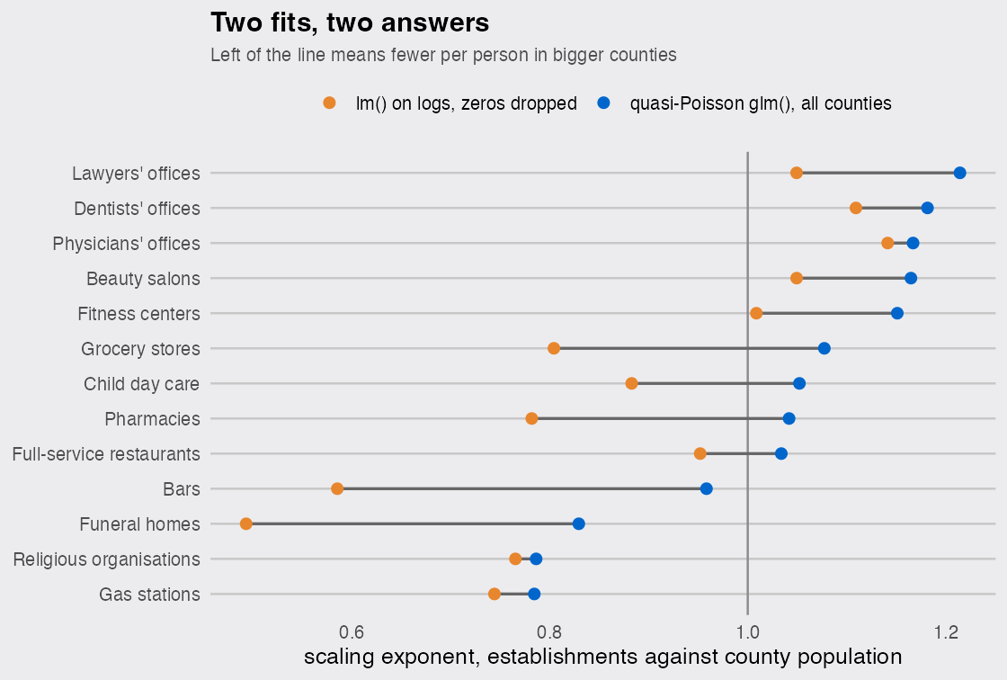
Across the thirteen industries the log-log fit is lower every time, by 0.14 on the median, and for 4 of them it lands on the other side of 1 and reverses the verdict: child day care, full-service restaurants, grocery stores, and pharmacies all look sublinear once the empty counties are gone and come out at or above proportional when they are kept. The industries where the two fits agree are the ones with almost no zeros to drop, like gas stations and religious organisations, which have an establishment in nearly every county.
Two things this exponent is not. Counties are administrative units rather than markets, so a county of 3,000 people with no grocery store is partly telling you that its residents shop in the next county over. And one exponent is a summary of a curve that need not be straight: funeral homes come out at 0.83, but their rate per person peaks in mid-sized counties, 0.65 per 10,000 in the middle decile against 0.13 at the bottom and 0.32 at the top. Plotting the per-person rate against population before reporting a single number is worth the extra line of code.


