How to detect heteroscedasticity and rectify it?

One of the important assumptions of linear regression is that, there should be no heteroscedasticity of residuals. In simpler terms, this means that the variance of residuals should not increase with fitted values of response variable. In this post, I am going to explain why it is important to check for heteroscedasticity, how to detect it in your model? If is present, how to make amends to rectify the problem, with example R codes. This process is sometimes referred to as residual analysis.

Why is it important to check for heteroscedasticity?

It is customary to check for heteroscedasticity of residuals once you build the linear regression model. The reason is, we want to check if the model thus built is unable to explain some pattern in the response variable \(Y\), that eventually shows up in the residuals. This would result in an inefficient and unstable regression model that could yield bizarre predictions later on.

How to detect heteroscedasticity?

I am going to illustrate this with an actual regression model based on the cars dataset, that comes built-in with R. Lets first build the model using the lm() function.

lmMod <- lm(dist ~ speed, data=cars) # initial model

Now that the model is ready, there are two ways to test for heterosedasticity:

• Graphically
• Through statistical tests

Graphical method

par(mfrow=c(2,2)) # init 4 charts in 1 panel
plot(lmMod)

Here it is the plot:

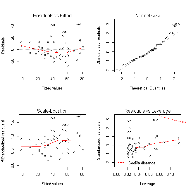
The plots we are interested in are at the top-left and bottom-left. The top-left is the chart of residuals vs fitted values, while in the bottom-left one, it is standardised residuals on Y axis. If there is absolutely no heteroscedastity, you should see a completely random, equal distribution of points throughout the range of X axis and a flat red line.

But in our case, as you can notice from the top-left plot, the red line is slightly curved and the residuals seem to increase as the fitted Y values increase. So, the inference here is, heteroscedasticity exists.

Statistical tests

Sometimes you may want an algorithmic approach to check for heteroscedasticity so that you can quantify its presence automatically and make amends. For this purpose, there are a couple of tests that comes handy to establish the presence or absence of heteroscedasticity – The Breush-Pagan test and the NCV test.

Breush Pagan Test

lmtest::bptest(lmMod)  # Breusch-Pagan test
	studentized Breusch-Pagan test

data:  lmMod
BP = 3.2149, df = 1, p-value = 0.07297

NCV Test

car::ncvTest(lmMod)  # Breusch-Pagan test
Non-constant Variance Score Test 
Variance formula: ~ fitted.values 
Chisquare = 4.650233    Df = 1     p = 0.03104933 

Both these test have a p-value less that a significance level of 0.05, therefore we can reject the null hypothesis that the variance of the residuals is constant and infer that heteroscedasticity is indeed present, thereby confirming our graphical inference.

How to rectify?

Re-build the model with new predictors.
Variable transformation such as Box-Cox transformation.

Since we have no other predictors apart from “speed”, I can’t show this method now. However, one option I might consider trying out is to add the residuals of the original model as a predictor and rebuild the regression model. With a model that includes residuals (as X) whose future actual values are unknown, you might ask what will be the value of the new predictor (i.e. residual) to use on the test data?. The solutions is, for starters, you could use the mean value of residuals for all observations in test data. Though is this not recommended, it is an approach you could try out if all available options fail. Lets now hop on to Box-Cox transformation.

Box-Cox transformation

Box-cox transformation is a mathematical transformation of the variable to make it approximate to a normal distribution. Often, doing a box-cox transformation of the Y variable solves the issue, which is exactly what I am going to do now.

distBCMod <- caret::BoxCoxTrans(cars$dist)
print(distBCMod)
Box-Cox Transformation

50 data points used to estimate Lambda

Input data summary:
   Min. 1st Qu.  Median    Mean 3rd Qu.    Max. 
   2.00   26.00   36.00   42.98   56.00  120.00 

Largest/Smallest: 60 
Sample Skewness: 0.759 

Estimated Lambda: 0.5

The model for creating the box-cox transformed variable is ready. Lets now apply it on car$dist and append it to a new dataframe.

cars <- cbind(cars, dist_new=predict(distBCMod, cars$dist)) # append the transformed variable to cars
head(cars) # view the top 6 rows
  speed dist  dist_new
1     4    2 0.8284271
2     4   10 4.3245553
3     7    4 2.0000000
4     7   22 7.3808315
5     8   16 6.0000000
6     9   10 4.3245553

The transformed data for our new regression model is ready. Lets build the model and check for heteroscedasticity.

lmMod_bc <- lm(dist_new ~ speed, data=cars)
bptest(lmMod_bc)
        studentized Breusch-Pagan test

data:  lmMod_bc
BP = 0.011192, df = 1, p-value = 0.9157

With a p-value of 0.91, we fail to reject the null hypothesis (that variance of residuals is constant) and therefore infer that ther residuals are homoscedastic. Lets check this graphically as well.

plot(lmMod_bc)

Here it is the plot:

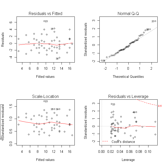
Ah, we have a much flatter line and an evenly distributed residuals in the top-left plot. So the problem of heteroscedsticity is solved and the case is closed. If you have any question post a comment below.