Classification algorithm defines set of rules to identify a category or group for an observation. There is various classification algorithm available like Logistic Regression, LDA, QDA, Random Forest, SVM etc. Here I am going to discuss Logistic regression, LDA, and QDA. The classification model is evaluated by confusion matrix. This matrix is represented by a table of Predicted True/False value with Actual True/False Value. The confusion matrix is shown as below. This list down the TRUE/FALSE for Predicted and Actual Value in a 2X2 table.
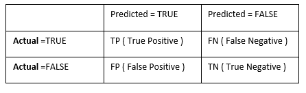
From the above table, prediction result is correct for TP and TN and prediction fails for FN and FP. Following terms are defined for confusion matrix:
- True Positive Rate = TP / ( TP+FN ) – Defines proportion of TRUE (Actual=TRUE) observations that are predicted ( predicted as TRUE ) correctly.
True Negative Rate = TN / ( TN+FP ) – Defines proportion of FALSE ( Actual=FALSE ) observations that are predicted ( predicted as FALSE ) correctly.
Accuracy = TP+TN / (TP+TN+FP+FN) – Defines overall correct prediction result.
Classification Algorithm (Logistic regression, LDA & QDA)
Logistic Regression
Logistic Regression is an extension of linear regression to predict qualitative response for an observation. It defines the probability of an observation belonging to a category or group. Logistics regression is generally used for binomial classification but it can be used for multiple classifications as well.
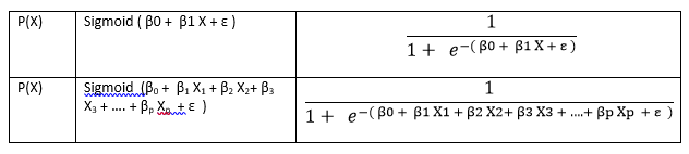
Following is the equation for linear regression for simple and multiple regression.
- Y = β0 + β1 X + ε ( for simple regression )
Y = β0 + β1 X1 + β2 X2+ β3 X3 + …. + βp Xp + ε (for multiple regression )
Linear Regression works for continuous data, so Y value will extend beyond [0,1] range. As the output of logistic regression is probability, response variable should be in the range [0,1]. To solve this restriction, the Sigmoid function is used over Linear regression to make the equation work as Logistic Regression as shown below.
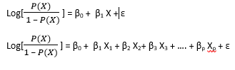
The above probability function can be derived as function of LOG (Log Odds to be more specific) as below. From the equation it is evident that Log odd is linearly related to input X. The Log Odd equation helps in better intuition of what will happen for a unit change in input (X1, X2…, Xp) value. For example – a change in one unit of predictor X1, and keeping all other predictor constant, will cause the change in the Log Odds of probability by β1 (Associated co-efficient of X1)
Bayes Theorem, LDA (Linear Discriminant Analysis) & QDA (Quadratic Discriminant Analysis )
LDA and QDA algorithms are based on Bayes theorem and are different in their approach for classification from the Logistic Regression. In Logistic regression, it is possible to directly get the probability of an observation for a class (Y=k) for a particular observation (X=x). LDA and QDA algorithm is based on Bayes theorem and classification of an observation is done in following two steps.
- Identify the distribution for input X for each of the class (or groups ex Y=k1, k2, k3 etc )
Flip the distribution using Bayes theorem to calculate the probability Pr(Y=k|X=x)
Mathematically the equation as follows:
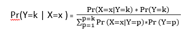
The above equation has following terms:
- Pr(Y=k|X=x) – Probability that an observation belongs to response class Y=k, provided X=x.
Pr(X=x|Y=k) – Probability of X=x, for a particular response class Y=k.
The distribution of X=x needs to be calculated from the historical data for every response class Y=k. In LDA algorithm, the distribution is assumed to be Gaussian and exact distribution is plotted by calculating the mean and variance from the historical data.
- Pr(Y=k) – a Prior probability that an observation is of particular class Y=k.
∑(Pr(X=x|Y=p)*Pr(Y=p)) – Sum of probability that an observation is of type X=x for all classes of Y.
In simple terms, if we need to identify a Disease (D1, D2,…, Dn) based on a set of symptoms (S1, S2,…, Sp) then from historical data, we need to identify the distribution of symptoms (S1, S2, .. Sp) for each of the disease ( D1, D2,…,Dn) and then using Bayes theorem it is possible to find the probability of the disease(say for D=D1) from the distribution of the symptom.
LDA (Linear Discriminant Analysis) is used when a linear boundary is required between classifiers and QDA (Quadratic Discriminant Analysis) is used to find a non-linear boundary between classifiers. LDA and QDA work better when the response classes are separable and distribution of X=x for all class is normal. The more the classes are separable and the more the distribution is normal, the better will be the classification result for LDA and QDA.
Following are the assumption required for LDA and QDA:
LDA Assumption:
- Common covariance across all response classes σ2 ( for ex σk1 = σk2 = σk3 for k1, k2 , k3 response classes )
Distribution of observation in each of the response classes is normal with a class-specific mean (µk) and common covariance σ.
QDA Assumption:
- Different covariance for each of the response classes. For ex – σk1, σk2, σk3 for response class k1, k2, k3 etc.
Distribution of observation in each of the response class is normal with a class-specific mean (µk) and class-specific covariance (σk2).
R Implementation
I will use the famous ‘Titanic Dataset’ available at Kaggle to compare the results for Logistic Regression, LDA and QDA.
Get the data and find the summary and dimension of the data
As a first step, we will check the summary and data-type. From the below summary we can summarize the following:
- Dataset has 891 rows and 12 columns.
Out of the 12 columns, we can remove PassengerId, Name and Ticket based on the UniqueValue dump from the dataset. The dump shows that the three features are mostly unique for passengers.
There is huge number of NA value for ‘Age’ (Almost 19.8 %, 177 out of 891) and so we can’t remove these rows. We will have a mechanism to replace the missing value for ‘Age’.
‘Cabin’ has huge number of missing value (687 out of 891) and so it will be better to not use this feature.
library(MASS)
library(ggplot2)
titanicDS = read.csv("train.csv")
dim(titanicDS)
[1] 891  12
str(titanicDS)
'data.frame':	891 obs. of  12 variables:
 $ PassengerId: int  1 2 3 4 5 6 7 8 9 10 ...
 $ Survived   : int  0 1 1 1 0 0 0 0 1 1 ...
 $ Pclass     : int  3 1 3 1 3 3 1 3 3 2 ...
 $ Name       : Factor w/ 891 levels "Abbing, Mr. Anthony",..: 109 191 358 277 16 559 520 629 417 581 ...
 $ Sex        : Factor w/ 2 levels "female","male": 2 1 1 1 2 2 2 2 1 1 ...
 $ Age        : num  22 38 26 35 35 NA 54 2 27 14 ...
 $ SibSp      : int  1 1 0 1 0 0 0 3 0 1 ...
 $ Parch      : int  0 0 0 0 0 0 0 1 2 0 ...
 $ Ticket     : Factor w/ 681 levels "110152","110413",..: 524 597 670 50 473 276 86 396 345 133 ...
 $ Fare       : num  7.25 71.28 7.92 53.1 8.05 ...
 $ Cabin      : Factor w/ 148 levels "","A10","A14",..: 1 83 1 57 1 1 131 1 1 1 ...
 $ Embarked   : Factor w/ 4 levels "","C","Q","S": 4 2 4 4 4 3 4 4 4 2 ...
summary(titanicDS)
  PassengerId       Survived          Pclass                                         Name
 Min.   :  1.0   Min.   :0.0000   Min.   :1.000   Abbing, Mr. Anthony                  :  1
 1st Qu.:223.5   1st Qu.:0.0000   1st Qu.:2.000   Abbott, Mr. Rossmore Edward          :  1
 Median :446.0   Median :0.0000   Median :3.000   Abbott, Mrs. Stanton (Rosa Hunt)     :  1
 Mean   :446.0   Mean   :0.3838   Mean   :2.309   Abelson, Mr. Samuel                  :  1
 3rd Qu.:668.5   3rd Qu.:1.0000   3rd Qu.:3.000   Abelson, Mrs. Samuel (Hannah Wizosky):  1
 Max.   :891.0   Max.   :1.0000   Max.   :3.000   Adahl, Mr. Mauritz Nils Martin       :  1
                                                  (Other)                              :885
     Sex           Age            SibSp           Parch             Ticket         Fare
 female:314   Min.   : 0.42   Min.   :0.000   Min.   :0.0000   1601    :  7   Min.   :  0.00
 male  :577   1st Qu.:20.12   1st Qu.:0.000   1st Qu.:0.0000   347082  :  7   1st Qu.:  7.91
              Median :28.00   Median :0.000   Median :0.0000   CA. 2343:  7   Median : 14.45
              Mean   :29.70   Mean   :0.523   Mean   :0.3816   3101295 :  6   Mean   : 32.20
              3rd Qu.:38.00   3rd Qu.:1.000   3rd Qu.:0.0000   347088  :  6   3rd Qu.: 31.00
              Max.   :80.00   Max.   :8.000   Max.   :6.0000   CA 2144 :  6   Max.   :512.33
              NA's   :177                                      (Other) :852
         Cabin     Embarked
            :687    :  2
 B96 B98    :  4   C:168
 C23 C25 C27:  4   Q: 77
 G6         :  4   S:644
 C22 C26    :  3
 D          :  3
 (Other)    :186
attach(titanicDS)
UniqueValue = function (x) {length(unique(x)) }
apply(titanicDS, 2, UniqueValue)
PassengerId    Survived      Pclass        Name         Sex         Age       SibSp
        891           2           3         891           2          89           7
      Parch      Ticket        Fare       Cabin    Embarked
          7         681         248         148           4
NaValue = function (x) {sum(is.na(x)) }
apply(titanicDS, 2, NaValue)
PassengerId    Survived      Pclass        Name         Sex         Age       SibSp
          0           0           0           0           0         177           0
      Parch      Ticket        Fare       Cabin    Embarked
          0           0           0           0           0
BlankValue = function (x) {sum(x=="") }
apply(titanicDS, 2, BlankValue)
PassengerId    Survived      Pclass        Name         Sex         Age       SibSp
          0           0           0           0           0          NA           0
      Parch      Ticket        Fare       Cabin    Embarked
          0           0           0         687           2
MissPercentage = function (x) {100 * sum (is.na(x)) / length (x) }
apply(titanicDS, 2, MissPercentage)
PassengerId    Survived      Pclass        Name         Sex         Age       SibSp
    0.00000     0.00000     0.00000     0.00000     0.00000    19.86532     0.00000
      Parch      Ticket        Fare       Cabin    Embarked
    0.00000     0.00000     0.00000     0.00000     0.00000
Process the missing value for ‘Age’.
The next step will be to process the ‘Age’ for the missing value. There are various ways to do this for example- delete the observation, update with mean, median etc. In the current dataset, I have updated the missing values in ‘Age’ with mean. Following code updates the ‘Age’ with the mean and so we can see that there is no missing value in the dataset.
titanicDS$Age[is.na(titanicDS$Age)] = mean(titanicDS$Age, na.rm=TRUE)
apply(titanicDS, 2, MissPercentage)
PassengerId    Survived      Pclass        Name         Sex         Age       SibSp
          0           0           0           0           0           0           0
      Parch      Ticket        Fare       Cabin    Embarked
          0           0           0           0           0
Now our data is data is ready to create the model. As a first step, we will split the data into testing and training observation. The data is split into 60-40 ratio and so there are 534 observation for training the model and 357 observation for evaluating the model.
set.seed(1)
row.number = sample(1:nrow(titanicDS), 0.6*nrow(titanicDS))
train = titanicDS[row.number,]
test = titanicDS[-row.number,]
dim(train)
dim(test)

[1] 534  12
[1] 357  12
Next, I will apply the Logistic regression, LDA, and QDA on the training data.
Logistic regression
Model1 – Initial model
We will make the model without PassengerId, Name, Ticket and Cabin as these features are user specific and have large missing value as explained above. From the ‘p’ value in ‘summary’ output, we can see that 4 features are significant and other are not statistically significant.
attach(train)
model1 = glm(factor(Survived)~.-PassengerId-Name-Ticket-Cabin, data=train, family=binomial)
summary(model1)
Call:
glm(formula = Survived ~ . - PassengerId - Name - Ticket - Cabin,
    family = binomial, data = train)

Deviance Residuals:
    Min       1Q   Median       3Q      Max
-2.5574  -0.6004  -0.4153   0.6457   2.4888

Coefficients:
              Estimate Std. Error z value Pr(>|z|)
(Intercept)  17.096211 535.411735   0.032   0.9745
Pclass       -1.034114   0.184390  -5.608 2.04e-08 ***
Sexmale      -2.700038   0.260657 -10.359  < 2e-16 ***
Age          -0.042137   0.009997  -4.215 2.50e-05 ***
SibSp        -0.299700   0.137998  -2.172   0.0299 *
Parch        -0.103531   0.158715  -0.652   0.5142
Fare          0.001456   0.003057   0.476   0.6338
EmbarkedC   -11.784667 535.411333  -0.022   0.9824
EmbarkedQ   -12.065422 535.411436  -0.023   0.9820
EmbarkedS   -12.460293 535.411309  -0.023   0.9814
---
Signif. codes:  0 ‘***’ 0.001 ‘**’ 0.01 ‘*’ 0.05 ‘.’ 0.1 ‘ ’ 1

(Dispersion parameter for binomial family taken to be 1)

    Null deviance: 706.29  on 533  degrees of freedom
Residual deviance: 469.52  on 524  degrees of freedom
AIC: 489.52

Number of Fisher Scoring iterations: 12
Model 2 – Remove the less significant feature.
As a next step, we will remove the less significant features from the model and we can see that out of 11 feature, 4 features are significant for model building.
#Remove Not significant features.
model2 = update(model1, ~.-Parch-Fare-Embarked)
summary(model2)
Call:
glm(formula = Survived ~ Pclass + Sex + Age + SibSp, family = binomial,
    data = train)

Deviance Residuals:
    Min       1Q   Median       3Q      Max
-2.6418  -0.6356  -0.4139   0.6333   2.4329

Coefficients:
             Estimate Std. Error z value Pr(>|z|)
(Intercept)  5.002039   0.603327   8.291  < 2e-16 ***
Pclass      -1.118165   0.153275  -7.295 2.98e-13 ***
Sexmale     -2.707990   0.249324 -10.861  < 2e-16 ***
Age         -0.041017   0.009798  -4.186 2.83e-05 ***
SibSp       -0.343279   0.131866  -2.603  0.00923 **
---
Signif. codes:  0 ‘***’ 0.001 ‘**’ 0.01 ‘*’ 0.05 ‘.’ 0.1 ‘ ’ 1

(Dispersion parameter for binomial family taken to be 1)

    Null deviance: 706.29  on 533  degrees of freedom
Residual deviance: 476.91  on 529  degrees of freedom
AIC: 486.91

Number of Fisher Scoring iterations: 5
Predict and get the accuracy of the model for training observation
The following dump shows the confusion matrix. Based on the confusion matrix, we can see that the accuracy of the model is 0.8146 = ((292+143)/534). Please note that we have fixed the threshold at 0.5 (probability = 0.5). It is possible to change the accuracy by fine-tuning the threshold (0.5) to a higher or lower value.
###Predict for training data and find training accuracy
pred.prob = predict(model2, type="response")
pred.prob = ifelse(pred.prob > 0.5, 1, 0)
table(pred.prob, Survived)
         Survived
pred.prob   0   1
        0 292  57
        1  42 143
Predict and get the accuracy of the model for test observation
Below we will predict the accuracy for the ‘test’ data, split in the first step in 60-40 ratio. Test data accuracy here is 0.7927 = (188+95)/357
##Predict for test Data and find the test accuracy.
attach(test)
pred.prob = predict(model2, newdata= test, type="response")
pred.prob = ifelse(pred.prob > 0.5, 1, 0)
table(pred.prob, Survived)
         Survived
pred.prob   0   1
        0 188  47
        1  27  95
LDA Model
We will use the same set of features that are used in Logistic regression and create the LDA model. The model has the following output as explained below:
- Prior probabilities of groups – This defines the prior probability of the response classes for an observation. This shows 36.14 % of the people survived and 63.8 % of people did not survive.
Group Means – This defines the mean value (µk) for response classes for a particular X=x. This indicates means values of different features when they fall to a particular response class. For example, we see a clear difference between the proportion of male (0.851 vs 0.31) for their survival class. The more the difference between mean, the easier it will be to classify observation.
Coefficients of the linear discriminants – This defines the coefficient of the linear equation that is used to classify the response classes. Note that in this model there are only two response classes and so there will be only one set of coefficients (LD1).
attach(train)
lda.model = lda (factor(Survived)~factor(Pclass)+Sex+Age+SibSp, data=train)
lda.model
lda.model
Call:
lda(factor(Survived) ~ factor(Pclass) + Sex + Age + SibSp, data = train)
Prior probabilities of groups:
        0         1
0.6254682 0.3745318

Group means:
  factor(Pclass)2 factor(Pclass)3   Sexmale      Age     SibSp
0       0.1736527       0.6736527 0.8413174 30.27826 0.5538922
1       0.2200000       0.3750000 0.3100000 27.87822 0.4900000

Coefficients of linear discriminants:
                        LD1
factor(Pclass)2 -0.87213055
factor(Pclass)3 -1.51560320
Sexmale         -2.14322979
Age             -0.02670928
SibSp           -0.19986406
As the next step, we will find the model accuracy for training data. Here we get the accuracy of 0.8033. This is little better than the Logistic Regression.
##Predicting training results.
predmodel.train.lda = predict(lda.model, data=train)
table(Predicted=predmodel.train.lda$class, Survived=Survived)
         Survived
Predicted   0   1
        0 290  61
        1  44 139
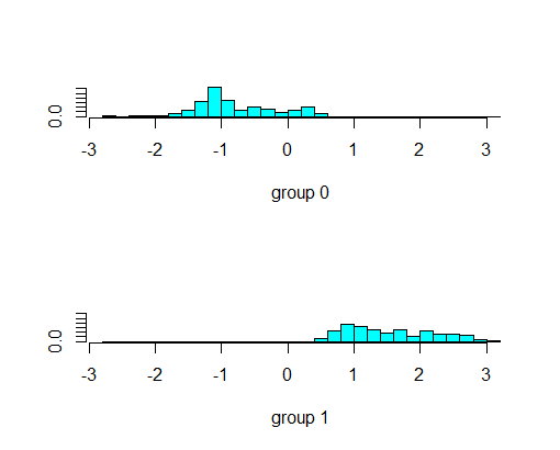
The below plot shows how the response class has been classified by the LDA classifier. The X-axis shows the value of line defined by the co-efficient of linear discriminant for LDA model. The two groups are the groups for response classes.
ldahist(predmodel.train.lda$x[,1], g= predmodel.train.lda$class)
Gives this plot:
Now we will check for model accuracy for test data 0.7983
attach(test)
predmodel.test.lda = predict(lda.model, newdata=test)
table(Predicted=predmodel.test.lda$class, Survived=test$Survived)
         Survived
Predicted   0   1
        0 189  46
        1  26  96
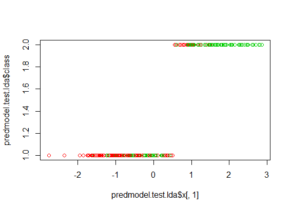
The below figure shows how the test data has been classified. The Predicted Group-1 and Group-2 has been colored with actual classification with red and green color. The mix of red and green color in the Group-1 and Group-2 shows the incorrect classification prediction.
par(mfrow=c(1,1))
plot(predmodel.test.lda$x[,1], predmodel.test.lda$class, col=test$Survived+10)
Gives this plot:
QDA Model
Next we will fit the model to QDA as below. The equation is same as LDA and it outputs the prior probabilities and Group means. Please note that ‘prior probability’ and ‘Group Means’ values are same as of LDA.
attach(train)
qda.model = qda (factor(Survived)~factor(Pclass)+Sex+Age+SibSp, data=train)
qda.model
> qda.model
Call:
qda(factor(Survived) ~ factor(Pclass) + Sex + Age + SibSp, data = train)

Prior probabilities of groups:
        0         1
0.6254682 0.3745318

Group means:
  factor(Pclass)2 factor(Pclass)3   Sexmale      Age     SibSp
0       0.1736527       0.6736527 0.8413174 30.27826 0.5538922
1       0.2200000       0.3750000 0.3100000 27.87822 0.4900000
In the next step, we will predict for training and test observation and check for their accuracy. Here training data accuracy: 0.8033 and testing accuracy is 0.7955.
##Predicting training results.
predmodel.train.qda = predict(qda.model, data=train)
table(Predicted=predmodel.train.qda$class, Survived=Survived)
         Survived
Predicted   0   1
        0 269  44
        1  65 156
##Predicting test results.
attach(test)
predmodel.test.qda = predict(qda.model, newdata=test)
table(Predicted=predmodel.test.qda$class, Survived=test$Survived)
         Survived
Predicted   0   1
        0 179  36
        1  36 106
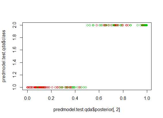
The below figure shows how the test data has been classified using the QDA model. The Predicted Group-1 and Group-2 has been colored with actual classification with red and green color. The mix of red and green color in the Group-1 and Group-2 shows the incorrect classification prediction.
par(mfrow=c(1,1))
plot(predmodel.test.qda$posterior[,2], predmodel.test.qda$class, col=test$Survived+10)
Gives this plot:
Conclusion
LDA and QDA work well when class separation and normality assumption holds true in the dataset. If the dataset is not normal then Logistic regression has an edge over LDA and QDA model. Logistic regression does not work properly if the response classes are fully separated from each other. In general, logistic regression is used for binomial classification and in case of multiple response classes, LDA and QDA are more popular.
Reference
1. Statistics for Business By Robert Stine, Dean Foster
2. An Introduction to Statistical Learning, with Application in R. By James, G., Witten, D., Hastie, T., Tibshirani, R.
2. An Introduction to Statistical Learning, with Application in R. By James, G., Witten, D., Hastie, T., Tibshirani, R.