
I went to Chicago’s traffic crash records to answer a small question: do crashes in bad weather injure more people than crashes in clear weather? The first answer I got back was that rain is safer than sunshine. That answer is wrong, and it was wrong for a reason that has nothing to do with weather. My request had returned 1,000 of the city’s 1.09 million crash records, and nothing in the response said so.
Chicago, New York, Seattle, Los Angeles and a few hundred other US agencies publish open data through Socrata, and every one of those endpoints truncates the same way. Here is how to see it happening, what it cost me, and the two ways past it.
Why does my Socrata API request return exactly 1,000 rows?
Because SoQL, the query language behind these endpoints, defaults $limit to 1,000. The response is an ordinary 200 carrying a complete-looking JSON array, so nothing marks it as partial. You have to ask for the row count as a separate query.
library(httr2)
library(dplyr)

crashes <- "https://data.cityofchicago.org/resource/85ca-t3if.json"

# a plain request, no query parameters
default_pull <- request(crashes) |>
  req_perform() |>
  resp_body_json(simplifyVector = TRUE) |>
  as_tibble()

nrow(default_pull)
## [1] 1000
# what is actually in the dataset
request(crashes) |>
  req_url_query(`$select` = "count(*)") |>
  req_perform() |>
  resp_body_json(simplifyVector = TRUE)
##     count
## 1 1091167
That is 0.09% of the data, retrieved with httr2 1.3.0 on 05 September 2026. The 1,000 rows are not the newest and not the oldest: mine ranged from 2017-03-18 to 2026-08-19, in an order the API does not document. They are also not a random sample you could put a confidence interval on, which turns out to matter.
What the missing 99.9% changes
On all 1,091,167 crashes, rain is the most injurious common weather condition and snow the least injurious. On the default 1,000 rows, both comparisons come out backwards.
The full answer costs one request, because SoQL will group and average on the server and send back a dozen rows instead of a million:
soda <- function(...) {
  request(crashes) |>
    req_url_query(...) |>
    req_perform() |>
    resp_body_json(simplifyVector = TRUE) |>
    as_tibble()
}

by_weather <- soda(
  `$select` = "weather_condition, count(*) AS n, avg(injuries_total) AS injuries,
               sum(injuries_fatal) AS fatal, stddev_pop(injuries_total) AS sd,
               avg(posted_speed_limit) AS speed",
  `$group`  = "weather_condition",
  `$order`  = "n DESC"
) |>
  mutate(across(c(n, injuries, fatal, sd, speed), as.numeric))

by_weather |> select(weather_condition, n, injuries, fatal)
## # A tibble: 12 × 4
##    weather_condition             n injuries fatal
##    <chr>                     <dbl>    <dbl> <dbl>
##  1 CLEAR                    856448   0.207   1030
##  2 RAIN                      90092   0.246    119
##  3 UNKNOWN                   67817   0.0668    23
##  4 SNOW                      35101   0.169     27
##  5 CLOUDY/OVERCAST           31933   0.212     28
##  6 OTHER                      3513   0.252      4
##  7 FREEZING RAIN/DRIZZLE      2572   0.234      2
##  8 FOG/SMOKE/HAZE             1623   0.255      2
##  9 SLEET/HAIL                 1230   0.234      0
## 10 BLOWING SNOW                630   0.266      2
## 11 SEVERE CROSS WIND GATE      186   0.176      1
## 12 BLOWING SAND, SOIL, DIRT     22   0.182      0
from_1k <- default_pull |>
  mutate(injuries_total = as.numeric(injuries_total)) |>
  group_by(weather_condition) |>
  summarise(n = n(), injuries = mean(injuries_total, na.rm = TRUE))
The UNKNOWN row is a reporting gap rather than a weather condition, and its very low injury count reflects thin crash reports, so I leave it out of the comparisons. Across every record, a crash in rain averages 0.246 reported injuries against 0.207 in clear weather, while a crash in snow averages 0.169, about a fifth below clear. Deaths agree with injuries: 1.32 fatalities per 1,000 rain crashes, 1.20 in clear weather and 0.77 in snow, so a snow crash is 36% less likely to kill someone than a clear-weather one. The posted speed limit is identical in the two (28.4 mph in snow, 28.4 in clear), so snow crashes are not simply happening on slower streets. Snow does not make crashes worse, it makes them slower, and it is rain, the condition drivers treat as ordinary, that shows up as the dangerous one.
None of that survives truncation. In my 1,000 rows, rain came out at 0.134 injuries per crash against 0.186 for clear, reversing the comparison, and the most injurious weather in Chicago appeared to be freezing rain/drizzle at 0.80 injuries per crash, computed from 5 rows.
library(ggplot2)

dsp_colors <- c("#0066CC", "#E8862D", "#159A6C", "#7D5BD6",
                "#D64580", "#2AA9B8", "#C9A227")
dsp_theme <- theme_minimal(base_size = 13) +
  theme(plot.background    = element_rect(fill = "#ECECEF", color = NA),
        panel.background   = element_rect(fill = "#ECECEF", color = NA),
        panel.grid.minor   = element_blank(),
        panel.grid.major.x = element_blank(),
        panel.grid.major.y = element_line(color = "grey78"),
        axis.ticks         = element_blank(),
        plot.title         = element_text(face = "bold"),
        strip.text         = element_text(face = "bold"))

keep <- c("CLEAR", "RAIN", "SNOW", "CLOUDY/OVERCAST", "FREEZING RAIN/DRIZZLE")
labs_src <- c(paste0("All ", format(n_total, big.mark = ","), " crashes"),
              "Default 1,000-row pull")

comparison <- bind_rows(
  by_weather |> select(weather_condition, injuries) |> mutate(src = labs_src[1]),
  from_1k    |> select(weather_condition, injuries) |> mutate(src = labs_src[2])
) |>
  filter(weather_condition %in% keep) |>
  mutate(weather_condition = factor(weather_condition, levels = keep),
         src = factor(src, levels = labs_src))

ggplot(comparison, aes(weather_condition, injuries, fill = src)) +
  geom_col(position = position_dodge(0.75), width = 0.68) +
  geom_text(aes(label = sprintf("%.2f", injuries)),
            position = position_dodge(0.75), vjust = -0.45,
            size = 3.4, color = "grey25") +
  scale_fill_manual(values = dsp_colors[1:2], name = NULL) +
  scale_x_discrete(labels = function(x) sub("/", "/\n", x)) +
  scale_y_continuous(expand = expansion(mult = c(0, 0.12))) +
  labs(title = "Injuries per crash by weather, Chicago",
       subtitle = "Truncating at 1,000 rows reverses rain and inflates rare conditions",
       x = NULL, y = "Injuries per crash") +
  dsp_theme +
  theme(legend.position = "top")
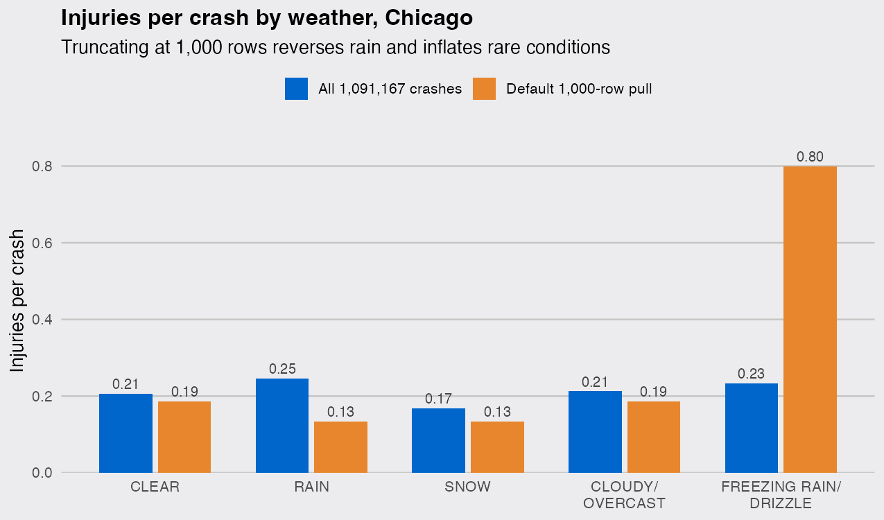
The truncated numbers are not so much biased as untethered. A 1,000-row pull leaves roughly 83 rain crashes in hand, and at that size the standard error on the rain-minus-clear difference is 0.073, nearly twice the 0.039 difference being measured. It takes about 13,900 rows before that standard error drops to half the gap. The danger is not that 1,000 rows is a small sample, it is that the response never says "sample", so nobody thinks to write down an error bar.
Getting all the rows, or not needing them
Two ways past the limit, and the second is usually the better one. If you need the individual records, raise $limit and walk the dataset with $offset until a page comes back short, ordering by the internal :id so the pages line up:
library(purrr)

read_all <- function(page = 1000, ...) {
  offset <- 0
  pages  <- list()
  repeat {
    pg <- soda(..., `$order` = ":id", `$limit` = page, `$offset` = offset)
    if (nrow(pg) == 0) break
    pages  <- append(pages, list(pg))
    offset <- offset + page
    if (nrow(pg) < page) break
  }
  list_rbind(pages)
}

snow_2025 <- read_all(
  `$select` = "crash_date, injuries_total, posted_speed_limit",
  `$where`  = "weather_condition = 'SNOW' AND crash_date >= '2025-01-01'"
)

nrow(snow_2025)
## [1] 6104
snow_recent <- mean(as.numeric(snow_2025$injuries_total), na.rm = TRUE)
snow_recent
## [1] 0.1967806
That is every snow crash Chicago has recorded since the start of 2025, 6,104 of them, averaging 0.197 injuries per crash.
If a summary is all you want, though, do not download rows in order to average them. $select with count(), avg(), sum() and stddev_pop() plus $group runs the aggregation on the server, and the whole recent-window comparison arrives in one request:
recent <- soda(
  `$select` = "weather_condition, count(*) AS n, avg(injuries_total) AS injuries",
  `$where`  = "crash_date >= '2025-01-01'",
  `$group`  = "weather_condition",
  `$order`  = "n DESC",
  `$limit`  = 5
) |>
  mutate(across(c(n, injuries), as.numeric))

recent
## # A tibble: 5 × 3
##   weather_condition      n injuries
##   <chr>              <dbl>    <dbl>
## 1 CLEAR             143982   0.244
## 2 UNKNOWN            15715   0.0792
## 3 RAIN               11163   0.296
## 4 SNOW                6104   0.197
## 5 CLOUDY/OVERCAST     5355   0.222
Reported injuries have risen across every condition lately, which is why that recent snow figure sits above the 0.169 of the full record rather than on top of it. The gap that matters is intact: snow runs 19% below clear weather in the 2025 data and 18% below it across all 1,091,167 crashes.
The habit worth keeping is the second query in this post. Any time an open data endpoint hands you a round number of rows, ask it for count(*) before you believe anything you compute.
