Card payments in a New York yellow cab end on a screen of tip buttons, usually 20%, 25% and 30%. I wanted to know what the 20% button actually charges. The city’s trip records hold the answer: every yellow-cab ride, published as one Parquet file per month. Twelve months is far too much to read into an R data frame on a laptop, and it does not need to be, because duckdb runs dplyr code on the files where they sit. The answer is that 20% means 20% of the whole bill, which on the median ride is 28% of the fare.
How do I query Parquet files in R that are too big to load?
Connect to an in-memory duckdb database and wrap read_parquet() in tbl(). You get a lazy table: dplyr verbs are translated to SQL, duckdb does the work, and only collect() brings rows into R. This block runs on its own with duckdb 1.5.5 and dbplyr 2.6.0 on R 4.6.1. It downloads the twelve monthly yellow taxi trip files from the Taxi and Limousine Commission (TLC) for August 2025 to July 2026, about 800 MB with no key needed, then counts every ride by how it was paid.
library(tidyverse)
library(duckdb)

dir.create("tlc", showWarnings = FALSE)
months <- format(seq(as.Date("2025-08-01"), by = "month", length.out = 12), "%Y-%m")
files <- file.path("tlc", paste0("yellow_tripdata_", months, ".parquet"))
urls <- paste0("https://d37ci6vzurychx.cloudfront.net/trip-data/", basename(files))
options(timeout = 600)
todo <- !file.exists(files)
walk2(urls[todo], files[todo], \(u, f) download.file(u, f, mode = "wb"))

con <- dbConnect(duckdb())
# union_by_name: the 2026 files gained a column, so match columns by name
trips <- tbl(con, sql("FROM read_parquet('tlc/*.parquet', union_by_name = true)"))

payments <- trips |>
  group_by(payment_type) |>
  summarise(rides = n(),
            tipped = mean(as.numeric(tip_amount > 0)),
            avg_tip = mean(tip_amount)) |>
  arrange(payment_type) |>
  collect() |>
  mutate(payment = c("Flex Fare", "Card", "Cash", "No charge",
                     "Dispute", "Unknown")[payment_type + 1], .before = 1)
payments
## # A tibble: 6 × 5
##   payment   payment_type    rides    tipped  avg_tip
##   <chr>            <dbl>    <dbl>     <dbl>    <dbl>
## 1 Flex Fare            0 11950045 0.0766    0.374
## 2 Card                 1 29990151 0.912     4.33
## 3 Cash                 2  4295331 0.0000610 0.000304
## 4 No charge            3   210517 0.000722  0.000547
## 5 Dispute              4   660848 0.000359  0.000449
## 6 Unknown              5        2 0         0
That is 47.1 million rides summarised in under a second; as an R data frame the same data would need about 8 GB of memory at 8 bytes a value. Two details in that code are worth knowing. mean(tip_amount > 0) fails on duckdb, which will not average TRUE and FALSE, so the logical goes through as.numeric() first. And duckdb can read the URLs directly instead of downloaded copies, but it fetches a remote file in many small range requests. After a year’s worth of those, the TLC’s server started answering 403 "Request blocked" for a few minutes. Downloading each file once is faster and kinder to the server.
Only card rides record tips reliably. The TLC’s data dictionary says cash tips are not included, and Flex Fare rides, booked in an app at an upfront price, show a tip on only 7.7% of trips. Everything below uses the 30.0 million card rides, 91.2% of which have a tip.
What does the 20% tip button in a New York taxi charge?
It charges 20% of the whole bill before the tip, meaning the fare plus surcharges, tax, the congestion charges and tolls, not 20% of the metered fare. Button tips are exact, which is what makes them visible in the data: a tip within 3 cents of 20, 25 or 30% of the bill is a button press. The tolerance covers Creative Mobile Technologies, one of the meter vendors, which rounds button amounts to the nearest 5 cents.
tipped <- trips |>
  filter(payment_type == 1, tip_amount > 0, fare_amount > 0) |>
  mutate(bill = total_amount - tip_amount,
         # Curb (vendor 2) leaves the airport fee out of its tip base
         bill = if_else(VendorID == 2, bill - coalesce(Airport_fee, 0), bill),
         pct = round(tip_amount / bill * 20) * 5,  # nearest multiple of 5%
         button = pct %in% c(20, 25, 30) &
                  abs(tip_amount - pct / 100 * bill) <= 0.03)

buttons <- tipped |>
  filter(button) |>
  group_by(pct) |>
  summarise(rides = n(),
            tip_share_of_fare = median(tip_amount / fare_amount),
            extras = median(bill - fare_amount),
            tips_on_extras = sum(pct / 100 * (bill - fare_amount))) |>
  arrange(pct) |>
  collect()
buttons
## # A tibble: 3 × 5
##     pct    rides tip_share_of_fare extras tips_on_extras
##   <dbl>    <dbl>             <dbl>  <dbl>          <dbl>
## 1    20 15262061             0.28    5         18432662.
## 2    25  2442478             0.348   4.75       3710275.
## 3    30   903462             0.425   4.75       1567463.
Of the 27.4 million tipped card rides, 68.0% land exactly on a button, and 55.8% on 20% alone. For comparison, 21% and 22% of the bill match 0.10% and 0.18% of tips, and the same button test run against the metered fare matches only 5.5%. The Curb line in the code came from trying both bases: on Curb airport pickups, 50% of tips are exactly 20% of the bill without the airport fee and 9% with it. Tolls are in the base for every vendor. The chart also shows smaller spikes at 10% and 15% of the bill, which could be other screen layouts or riders doing the arithmetic on the total shown; I count only the three standard buttons.
dsp_colors <- c("#0066CC", "#E8862D", "#159A6C", "#7D5BD6",
                "#D64580", "#2AA9B8", "#C9A227")
dsp_theme <- theme_minimal(base_size = 13) +
  theme(plot.background    = element_rect(fill = "#ECECEF", color = NA),
        panel.background   = element_rect(fill = "#ECECEF", color = NA),
        panel.grid.minor   = element_blank(),
        panel.grid.major.x = element_blank(),
        panel.grid.major.y = element_line(color = "grey78"),
        axis.ticks         = element_blank(),
        plot.title         = element_text(face = "bold"),
        strip.text         = element_text(face = "bold"))

shares <- tipped |>
  transmute(whole_bill = round(tip_amount / bill * 400) / 4,  # quarter-point bins
            fare = round(tip_amount / fare_amount * 400) / 4) |>
  pivot_longer(everything(), names_to = "base", values_to = "share") |>
  filter(share <= 50) |>
  count(base, share) |>
  collect() |>
  mutate(base = factor(base, levels = c("whole_bill", "fare"),
                       labels = c("Tip as % of the whole bill",
                                  "Tip as % of the metered fare")))

ggplot(shares, aes(share, n / 1e6)) +
  geom_col(fill = dsp_colors[1], width = 0.25) +
  facet_wrap(~ base, ncol = 1, scales = "free_y") +
  scale_x_continuous(breaks = seq(0, 50, 5)) +
  labs(x = "Tip (%)", y = "Card rides (millions)",
       title = "Card tips pile up on the buttons, measured against the whole bill") +
  dsp_theme
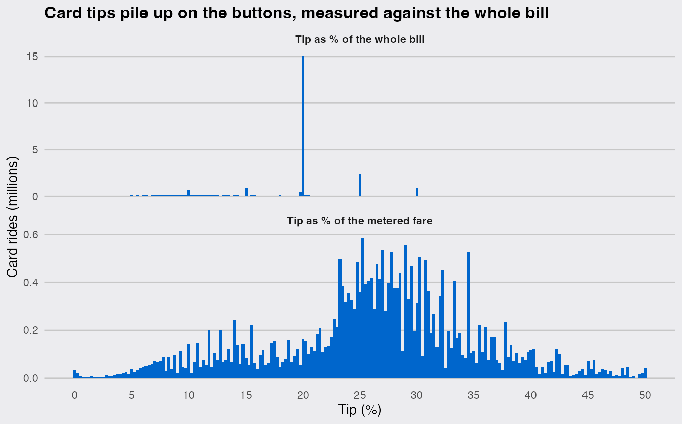
Measured against the fare, the same tips spread into a broad hump with nothing special at 20%, because the bill carries a median $5.00 on top of the fare. On the median ride the 20% button tips 28.0% of the fare, and on rides with a fare under $10, where the fixed charges weigh most, 33.8%. On a JFK flat-fare ride, $70 on the meter plus $6.94 in tolls at the median, the button adds $16.34 rather than $14. Over the twelve months, button presses put $23.7 million of tips on the extras, 18% of every tip recorded on a card.
Why does == undercount the button tips?
Testing tip_amount == 0.2 * bill finds only 27.6% of tipped rides at 20%, about half the real 55.8%. Most amounts in cents have no exact binary representation, so the product is off in the 16th digit and the equality fails:
0.2 * 18.55 == 3.71
## [1] FALSE
sprintf("%.17f", 0.2 * 18.55)
## [1] "3.71000000000000041"
Compare money with a tolerance, as in the button test, or round both sides to cents first.
So in a New York yellow cab, 20% means 20% of everything on the bill, which on the median ride is 28% of the fare, and across a year of rides it added $23.7 million of tips on surcharges, tax and tolls. On the R side, a folder of Parquet files, duckdb and ordinary dplyr code were enough to get there from 47.1 million rows on a laptop.


