
There is a routine that shows up almost everywhere linear regression is taught: fit the model, plot residuals against fitted values, run a Breusch-Pagan test, and if the p-value is small, transform the outcome and refit. I wanted to look at the two steps in the middle, because both of them hide something.
The first is the test itself. R gives you two implementations of the Breusch-Pagan test, they get used interchangeably, and only one of them is really a test for non-constant variance. The other also reacts to the shape of the error distribution: on data with heavy tails and perfectly constant variance, it rejects about half the time.
The second is what happens after. A significant test tells you the model has a problem somewhere, but it says nothing about which coefficient is damaged or by how much. On the data below, one coefficient’s standard error is off by 7% and another by 100%, from the same single p-value.
So this post is about closing that gap: what the test measures, what the fix actually changes, and which robust variance estimator to reach for. Everything runs on lmtest, sandwich and the tidyverse.
A model with a very obvious problem
I used the Ames housing data that ships with the modeldata package: every residential sale in Ames, Iowa between 2006 and 2010, with the lot and building characteristics recorded for each one. I kept the ordinary arm’s-length sales and regressed the sale price on four measurements a buyer can see.
library(tidyverse)
library(modeldata)
library(lmtest)
library(sandwich)
library(broom)

data(ames)

homes <- ames |>
  filter(Sale_Condition == "Normal") |>
  transmute(price      = Sale_Price / 1000,   # thousands of dollars
            area       = Gr_Liv_Area,         # above-grade living area, sq ft
            year_built = Year_Built,
            lot        = Lot_Area / 1000,     # thousands of sq ft
            basement   = Total_Bsmt_SF)

fit <- lm(price ~ area + year_built + lot + basement, data = homes)
nrow(homes)
## [1] 2413
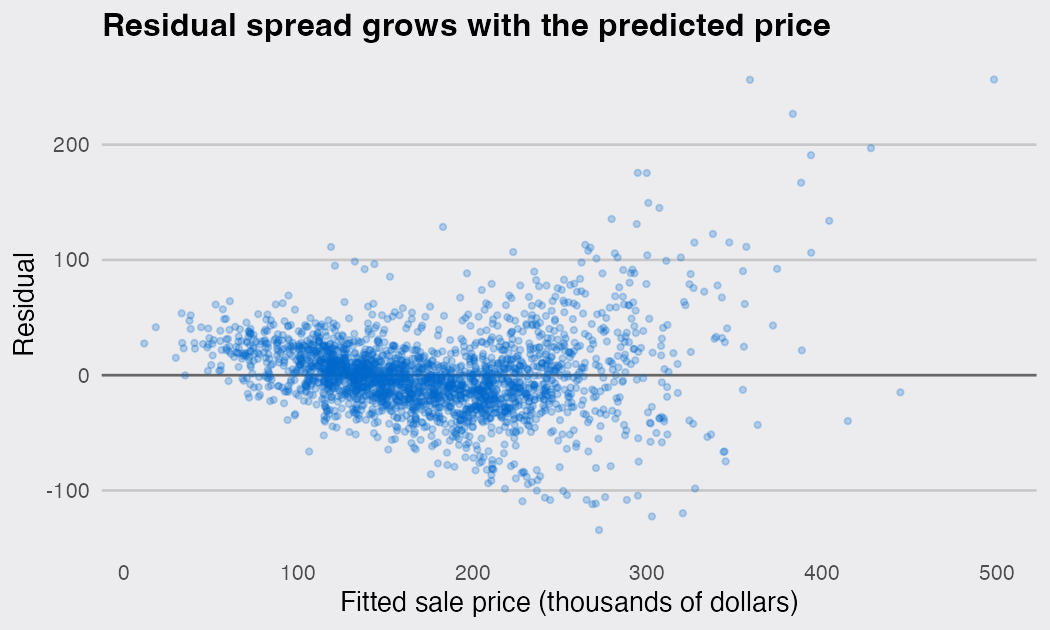
That leaves 2,413 sales. The residual plot is the textbook picture, so much so that it barely needs a test:
dsp_colors <- c("#0066CC", "#E8862D", "#159A6C", "#7D5BD6",
                "#D64580", "#2AA9B8", "#C9A227")
dsp_theme <- theme_minimal(base_size = 13) +
  theme(plot.background    = element_rect(fill = "#ECECEF", color = NA),
        panel.background   = element_rect(fill = "#ECECEF", color = NA),
        panel.grid.minor   = element_blank(),
        panel.grid.major.x = element_blank(),
        panel.grid.major.y = element_line(color = "grey78"),
        axis.ticks         = element_blank(),
        plot.title         = element_text(face = "bold"),
        strip.text         = element_text(face = "bold"))

augment(fit) |>
  ggplot(aes(.fitted, .resid)) +
  geom_hline(yintercept = 0, color = "grey40") +
  geom_point(alpha = 0.25, size = 1.1, color = dsp_colors[1]) +
  labs(title = "Residual spread grows with the predicted price",
       x = "Fitted sale price (thousands of dollars)", y = "Residual") +
  dsp_theme
(That theme snippet is reusable, so copy it once and drop it on every figure in a post.)
Cheap houses are predicted to within a few thousand dollars; expensive ones miss by a hundred thousand in either direction. The test agrees, emphatically:
bptest(fit)
##
## 	studentized Breusch-Pagan test
##
## data:  fit
## BP = 440.22, df = 4, p-value < 2.2e-16
What the test is reacting to
Here is the part that is easy to miss. There are two Breusch-Pagan tests in common use in R, and they are not the same test.
The original 1979 statistic regresses the squared residuals on the predictors and scales the result by a variance figure that only holds if the errors are normal. bptest(fit, studentize = FALSE) computes exactly that, and car::ncvTest() computes the same normality-dependent score test (scored against the fitted values rather than the predictors, by default). The studentized version, from Koenker (1981), replaces the assumed scale with one estimated from the residuals, which makes it valid whatever the error distribution looks like. lmtest::bptest() uses the studentized version by default, which is why its printed heading says "studentized Breusch-Pagan test".
The difference matters more than the naming suggests. To see how much, I generated data where the variance really is constant, varied only the shape of the error distribution, and counted how often each version rejects at the 5% level. Every rejection in that setting is a false alarm. I then repeated it with variance that genuinely grows with x, where rejections are the desired outcome.
n <- 200
x <- rnorm(n)

errors <- function(shape) {
  e <- switch(shape,
              "normal"     = rnorm(n),
              "t(5)"       = rt(n, df = 5),
              "log-normal" = exp(rnorm(n)),
              "uniform"    = runif(n))
  (e - mean(e)) / sd(e)          # same variance, different shape
}

one_run <- function(shape, variance) {
  spread <- if (variance == "constant variance") 1 else exp(0.15 * x)
  y <- 1 + x + errors(shape) * spread
  m <- lm(y ~ x)
  tibble(shape = shape, variance = variance,
         studentized = bptest(m)$p.value,
         original    = bptest(m, studentize = FALSE)$p.value)
}

grid <- expand_grid(shape    = c("normal", "t(5)", "log-normal", "uniform"),
                    variance = c("constant variance", "variance grows with x"),
                    rep      = 1:2000)

rates <- pmap_dfr(list(grid$shape, grid$variance), one_run) |>
  pivot_longer(c(studentized, original), names_to = "test", values_to = "p") |>
  group_by(variance, shape, test) |>
  summarise(reject = mean(p < 0.05), .groups = "drop")

rates |> pivot_wider(names_from = test, values_from = reject)
## # A tibble: 8 × 4
##   variance              shape      original studentized
##   <chr>                 <chr>         <dbl>       <dbl>
## 1 constant variance     log-normal   0.525       0.05
## 2 constant variance     normal       0.046       0.0495
## 3 constant variance     t(5)         0.187       0.046
## 4 constant variance     uniform      0.0025      0.0495
## 5 variance grows with x log-normal   0.630       0.124
## 6 variance grows with x normal       0.800       0.795
## 7 variance grows with x t(5)         0.709       0.482
## 8 variance grows with x uniform      0.91        0.990
rates |>
  mutate(shape = factor(shape, c("uniform", "normal", "t(5)", "log-normal"))) |>
  ggplot(aes(shape, reject, fill = test)) +
  geom_col(position = position_dodge(width = 0.7), width = 0.6) +
  geom_hline(yintercept = 0.05, linetype = "dashed", color = "grey30") +
  facet_wrap(~ variance) +
  scale_fill_manual(values = dsp_colors[c(2, 1)], name = NULL,
                    labels = c("original (assumes normality)",
                               "studentized (bptest default)")) +
  scale_y_continuous(labels = scales::percent) +
  labs(title = "In the left panel, every rejection is a false alarm",
       subtitle = "Rejection rate at the 5% level, 2,000 simulations per bar",
       x = "Error distribution", y = "Rejections at the 5% level") +
  dsp_theme +
  theme(legend.position = "top")
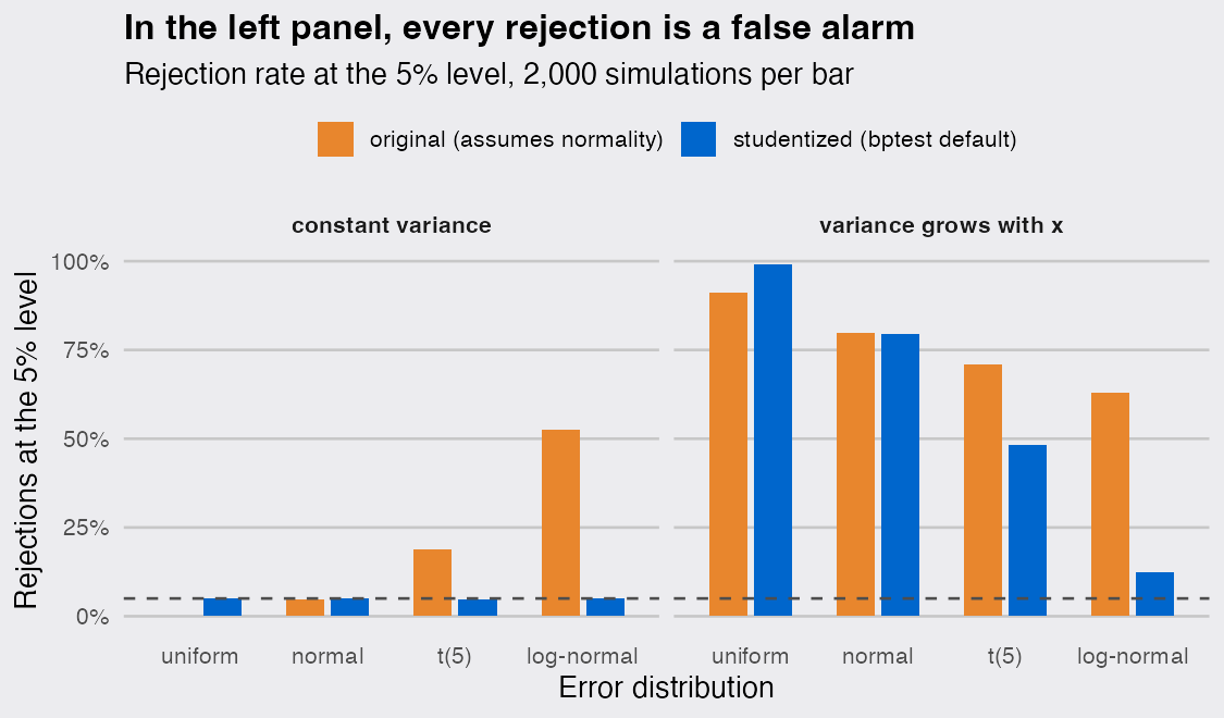
Read the left panel first. With normally distributed errors both versions behave, sitting on the dashed 5% line. Swap in log-normal errors and the original test rejects 52% of the time, even though the variance never changes. Student’s t with 5 degrees of freedom, a mild amount of extra tail weight, gets it to 19%. The studentized version stays near 5% throughout.
The failure runs in the other direction too. With light-tailed uniform errors the original test rejects almost never under the null, 0.2%, which is not caution but a broken calibration that costs it detections elsewhere.
The reason is that the original statistic divides by a variance figure that is only correct when the errors are normal. Heavy tails inflate the squared residuals it is testing without inflating that denominator, so kurtosis reads as heteroscedasticity. Studentizing estimates the denominator from the residuals instead, and the sensitivity to shape disappears.
Now the right panel, where the variance really does grow with x. With normal errors the two versions have essentially identical power (80% against 80%), so the protection in the left panel is free. But look at the log-normal bars: the studentized test finds real heteroscedasticity only 12% of the time. Its higher-looking neighbor is not better, because a test that fires 52% of the time under the null cannot have its rejections interpreted.
That is the practical takeaway from this section, and it has two halves. Use the studentized version, which is what you get by default from bptest(). And do not read a non-significant result as a clean bill of health, because with skewed or heavy-tailed errors the honest test has very little power.
What robust standard errors actually change
Back to the houses, where the test result was not in doubt anyway. The usual next move is to transform the outcome, but that changes the quantity being estimated: a coefficient in a log-price model is a percentage effect, not a dollar effect, and if the dollar effect is what you wanted, you have answered a different question to fix a standard error.
The alternative keeps the model and fixes only the standard errors. sandwich::vcovHC() builds a heteroscedasticity-consistent covariance matrix, and coeftest() re-runs the coefficient table with it.
comparison <- bind_rows(
  classical = tidy(fit),
  HC3       = tidy(coeftest(fit, vcov. = vcovHC(fit))),
  .id = "vcov") |>
  filter(term != "(Intercept)") |>
  select(vcov, term, estimate, std.error, statistic) |>
  pivot_wider(names_from = vcov, values_from = c(std.error, statistic)) |>
  mutate(inflation = std.error_HC3 / std.error_classical)

print(comparison, width = Inf)
## # A tibble: 4 × 7
##   term       estimate std.error_classical std.error_HC3 statistic_classical
##   <chr>         <dbl>               <dbl>         <dbl>               <dbl>
## 1 area         0.0786             0.00159       0.00254               49.4
## 2 year_built   0.731              0.0257        0.0275                28.5
## 3 lot          0.685              0.0881        0.176                  7.78
## 4 basement     0.0521             0.00198       0.00303               26.4
##   statistic_HC3 inflation
##           <dbl>     <dbl>
## 1         30.9       1.60
## 2         26.5       1.07
## 3          3.90      2.00
## 4         17.2       1.53
The point estimates never move, because ordinary least squares is still unbiased under heteroscedasticity. Only the uncertainty around them changes, and this is where a single global p-value stops being useful. The inflation factor runs from 1.07 on year_built to 2.00 on lot. The year the house was built has a standard error that was essentially fine all along. The lot size coefficient had a standard error half the size it should be, and its t statistic falls from 7.8 to 3.9.
Why that coefficient? Because heteroscedasticity only distorts a standard error where the large errors coincide with the extreme values of that predictor, and lot size is the variable with the extremes:
c(median_lot = median(homes$lot), largest_lot = max(homes$lot))
##  median_lot largest_lot
##       9.360     215.245
# how much of the lot-size variation comes from ten properties
big <- slice_max(homes, lot, n = 10)
sum((big$lot - mean(homes$lot))^2) / sum((homes$lot - mean(homes$lot))^2)
## [1] 0.6923105
c(mean_leverage = mean(hatvalues(fit)), max_leverage = max(hatvalues(fit)))
## mean_leverage  max_leverage
##   0.002072109   0.270229368
A handful of acreages, one of them 23 times the median lot, carry most of the information about that slope, and those same properties have the largest residuals. That is the worst possible combination, and it is invisible in the omnibus test.
One more thing worth knowing, because "robust" is often heard as "conservative": the correction is not guaranteed to make standard errors bigger. When the largest errors sit in the middle of a predictor’s range rather than at its extremes, it goes the other way.
ratio <- replicate(1000, {
  x <- rnorm(300)
  y <- 1 + x + rnorm(300, sd = exp(-0.6 * abs(x)))  # noisiest near the center
  m <- lm(y ~ x)
  sqrt(diag(vcovHC(m)))[["x"]] / sqrt(diag(vcov(m)))[["x"]]
})
c(mean_ratio = mean(ratio), share_below_one = mean(ratio < 1))
##      mean_ratio share_below_one
##       0.6535694       1.0000000
Every simulated dataset gets a smaller robust standard error, averaging 0.65 times the classical one. The sandwich estimator is not a safety margin bolted on top of the classical one. It is a different estimate, and it can point either way.
Which sandwich
vcovHC() offers several corrections, and the choice matters far more than it appears to. HC0 is the original White estimator. HC1 applies a degrees-of-freedom factor and is what Stata’s robust option reports. HC3 divides each squared residual by (1 - h)², where h is that observation’s leverage, which approximates what you would get by leaving the point out and refitting. To see what that buys, I simulated data with real heteroscedasticity and measured how often a nominal 95% interval for the slope actually contains the true value.
covers <- function(m, V, truth = 1) {
  ci <- coefci(m, vcov. = V)["x", ]
  ci[1] <= truth & truth <= ci[2]
}

one_fit <- function(n) {
  x <- rnorm(n)
  y <- 1 + x + rnorm(n, sd = exp(0.6 * x))
  m <- lm(y ~ x)
  tibble(n = n,
         classical = covers(m, vcov(m)),
         HC0 = covers(m, vcovHC(m, type = "HC0")),
         HC1 = covers(m, vcovHC(m, type = "HC1")),
         HC3 = covers(m, vcovHC(m, type = "HC3")))
}

sizes <- c(30, 60, 120, 500)

cover <- map_dfr(rep(sizes, each = 2000), one_fit) |>
  pivot_longer(-n, names_to = "vcov", values_to = "covered") |>
  group_by(n, vcov) |>
  summarise(coverage = mean(covered), .groups = "drop")

cover |> pivot_wider(names_from = vcov, values_from = coverage)
## # A tibble: 4 × 5
##       n   HC0   HC1   HC3 classical
##   <dbl> <dbl> <dbl> <dbl>     <dbl>
## 1    30 0.898 0.912 0.953     0.828
## 2    60 0.918 0.922 0.940     0.820
## 3   120 0.934 0.936 0.942     0.815
## 4   500 0.946 0.946 0.951     0.79
cover |>
  ggplot(aes(factor(n), coverage, color = vcov, group = vcov)) +
  geom_hline(yintercept = 0.95, linetype = "dashed", color = "grey30") +
  geom_line(linewidth = 0.9) +
  geom_point(size = 2.4) +
  scale_y_continuous(labels = scales::percent, limits = c(0.75, 1)) +
  scale_color_manual(values = dsp_colors[c(5, 2, 7, 3)], name = NULL) +
  labs(title = "Coverage of a nominal 95% interval for the slope",
       subtitle = "2,000 simulations per point, variance growing with x",
       x = "Sample size", y = "Coverage") +
  dsp_theme +
  theme(legend.position = "top")
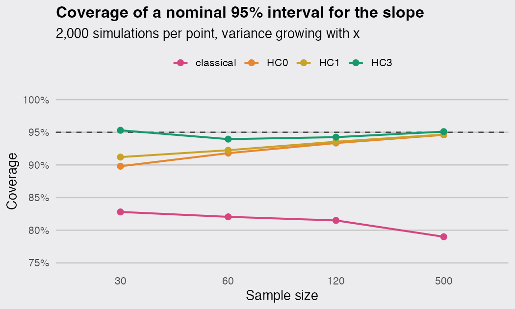
The classical interval is the flat line at the bottom, covering around 81% instead of 95%, and it gets worse as the sample grows. That is the thing to internalize about heteroscedasticity: it is not a small-sample problem that more data will wash out. The interval is converging, just to the wrong width.
Among the robust options, at n = 500 they are indistinguishable, which is the textbook claim and the reason the choice often gets waved through. At n = 30 they are not: HC0 covers 89.8% and HC1 91.2%, while HC3 reaches 95.3%. A test you believe runs at 5% is running closer to 10%. HC3 is the default in vcovHC() for exactly this reason, so plain vcovHC(fit) is already the right call, and the way to get this wrong is to type a type = argument copied from somewhere else.
The routine I would use instead
Plot the residuals, always. The picture tells you the shape of the problem, which no p-value does.
Run bptest() and leave studentize alone, and treat a non-significant result as weak evidence rather than as clearance, especially when the residuals are skewed.
Skip the test as a gate on whether to use robust standard errors. Deciding between two covariance estimators by looking at a p-value from the same data makes the reported standard error a random choice between them, and the heteroscedasticity-consistent one is valid either way, costing only a little efficiency when the variance really is constant. Report coeftest(fit, vcov. = vcovHC(fit)) and be done.
Transform the outcome when the transformed scale is the one you want to interpret, not as a repair for a standard error.
And when a coefficient’s standard error moves a lot under the correction, go look at that predictor. On the Ames data the correction was not just a technical adjustment: it pointed at ten properties that were quietly running the lot-size coefficient.
