One of the assumptions of Classical Linear Regression Model is that there is no exact collinearity between the explanatory variables. If the explanatory variables are perfectly correlated, you will face with these problems:
- Parameters of the model become indeterminate
- Standard errors of the estimates become infinitely large
However, the case of perfect collinearity is very rare in practical cases. Imperfect or less than perfect multicollinearity is the more common problem and it arises when in multiple regression modelling two or more of the explanatory variables are approximately linearly related.
The consequences are:
- OLS estimators are still unbiased, but they have large variances and covariances, making precise estimation difficult
- As a result, the confidence intervals tend to be wider. Therefore, we may not reject the “zero null hypothesis” (i.e. the true population coefficient is zero)
- Because of first consequence, the t ratios of one or more coefficients tend to be statistically insignificant
- Even though some regression coefficients are statistically insignificant, the \(R^2 \) value may be very high
- The OLS estimators and their standard errors can be sensitive to small changes in the data
So, it is must to detect the collinearity as well as to remove them. The collinearity can be detected in the following ways:
- The The easiest way for the detection of multicollinearity is to examine the correlation between each pair of explanatory variables. If two of the variables are highly correlated, then this may the possible source of multicollinearity. However, pair-wise correlation between the explanatory variables may be considered as the sufficient, but not the necessary condition for the multicollinearity.
- The second easy way for detecting the multicollinearity is to estimate the multiple regression and then examine the output carefully. The rule of thumb to doubt about the presence of multicollinearity is very high \(R^2 \) but most of the coefficients are not significant according to their p-values. However, this cannot be considered as an acid test for detecting multicollinearity. It will provide an apparent idea for the presence of multicollinearity.
- As, the coefficient of determination in the regression of regressor \(X_j\) on the remaining regressors in the model, increases toward unity, that is, as the collinearity of \(X_j\) with the other regressors increases, \(VIF \) also increases and in the limit it can be infinite. Therefore, we can use the \(VIF \) as an indicator of multicollinearity. The larger the value of \(VIF_j \), the more “troublesome” or collinear the variable \(X_j \). As a rule of thumb, if the \(VIF \) of a variable exceeds 10, which will happen if multiple correlation coefficient for j-th variable \(R_j^2 \) exceeds 0.90, that variable is said to be highly collinear.
- The Farrar-Glauber test (F-G test) for multicollinearity is the best way to deal with the problem of multicollinearity.
The F-G test is, in fact, a set of three tests for testing multicollinearity
- Firstly, a Chi-square test for the detection of the existence and severity of multicollinearity is a function with several explanatory variables. The hypothesis to be tested in the first step is:
$$ H_0 : \text {the X’s are orthogonal} \\
against\\
H_1: \text {the X’s are not orthogonal} $$
The variables are standardised for the sample size and standard deviation. Using the standardised explanatory variables, a standardised determinant is formed. This standardised determinant, also called as correlation determinant, is written in a form keeping in mind that the main diagonal elements are equal to unity and the off-diagonal elements are the simple correlation coefficients among the explanatory variables. The standardised determinant for three variables case is written as
$$ \begin{vmatrix}
1 & r_{x_1 x_2} & r_{x_1 x_3} \\
r_{x_1 x_2} & 1 & r_{x_2 x_3} \\
r_{x_1 x_3} & r_{x_2 x_3} & 1
\end{vmatrix} $$
Now in case of perfect multicollinearity the simple correlation coefficients are equal to unity and so the above determinant turns to zero. That is,
$$ \begin{vmatrix}
1 & 1 & 1 \\
1 & 1 & 1 \\
1 & 1 & 1
\end{vmatrix} =0 $$
On the other hand, in case of orthogonality of the explanatory variables the simple correlation coefficients are all equal to zero and so the standardized determinant turns to unity. That is,
$$ \begin{vmatrix}
1 & 0 & 0 \\
0 & 1 & 0 \\
0 & 0 & 1
\end{vmatrix} =1 $$
In practice, however, as either the perfect multicollinearity or orthogonality is very rare, the above determinant lies between zero and unity, and there is some degree of multicollinearity in the model.
Thus, the problem of multicollinearity may be considered as the departure from the orthogonality. The stronger the departure from the orthogonality (or the closer the value of the standardized determinant to zero), the stronger the degree of multicollinearity and vice versa.
From this notion Farrar and Glauber have developed the Chi-square test for detecting the strength of the multicollinearity over the whole set of explanatory variables. The Chi-square test statistic is given by
$$ \chi^2 = – \left [n-1 \frac 1 6 \left (2k+5 \right) \right].log_e [\text {value of the determinant}] $$
Under the assumption of true null hypothesis, the test statistic will follow a Chi-square distribution with \(df=\frac 1 2 k(k-1)\)If the observed value of the Chi-square test statistic is found to be greater than the critical value of Chi-square at the desired level of significance, we reject the assumption of orthogonality and accept the presence of multicollinearity in the model.
If the observed value of the Chi-square test statistic is found to be less than the critical value of Chi-square at the desired level of significance, we accept that there is no problem of multicollinearity in the model. - The second test in the Farar-Glauber test is an F test for the location of multicollinearity. To do this, they have computed the multiple correlation coefficients among the explanatory variablesand tested the statistical significance of these multiple correlation coefficients using an F test. The test statistic is given as
$$F = \frac {\left (R_{x_1.x_2 x_3 ….x_k}^2 \right)/(k-1)}{\left (1-R_{x_1.x_2 x_3 ….x_k}^2\right)/(n-k)}$$
where \(n=\text {sample size}\) and \(k=\text {number of explanatory variables}\)The hypothesis to be tested is given as
$$H_0 : R_{x_1 .x_2 x_2 …..x_k}^2=0 \\ H_1: R_{x_1 .x_2 x_2 …..x_k}^2 \neq 0$$If the observed value of \(F\) is found to be greater than the theoretical value of \(F\) with degrees of freedom at the desired level of significance, we accept that the variable \(X_i\) multicollinear.
On the other hand, if the observed value of \(F\) is less than the theoretical value of \(F\), we accept that the variable \(X_i\) is not multicollinear.
You should note that there will as many number of \(F\) test as the number of explanatory variables present in the model. - Finally, the Farrar – Glauber test concludes with a t – test for the pattern of multicollinearity. In fact, this is a t-test which aims at the detection of the variables which cause multicollinearity. To do this, the partial correlation coefficients among the explanatory variables are computed and their statistical significance are tested with the t test. For the above three variables modelling, the partial correlation coefficients are given by the formula
$$ r_{x_1 x_2 .x_3}^2 = \frac {\left (r_{12} – r_{13}r_{23} \right)^2}{\left (1-r_{23}^2\right) \left (1- r_{13}^2\right) } \\r_{x_1 x_3 .x_2}^2 = \frac {\left (r_{13} – r_{12}r_{23} \right)^2}{\left (1-r_{23}^2\right) \left (1- r_{12}^2\right) } \\r_{x_1 x_2 .x_3}^2 = \frac {\left (r_{23} – r_{12}r_{13} \right)^2}{\left (1-r_{13}^2\right) \left (1- r_{12}^2\right) } $$
For the statistical model involving more than three explanatory variables, we can develop similar formula for partial correlation coefficients.
The hypothesis to be tested at this step is as under:
$$ H_0 : r_{x_i x_j . x_1 x_2 ….x_k} = 0 \\ H_0 : r_{x_i x_j . x_1 x_2 ….x_k} \neq 0 $$
After calculating all the partial correlation coefficients, their statistical significance are tested individually for each of them by using the following test statistic
$$ t= \frac {\left (r_{x_i x_j . x_1 x_2…..x_k}\right )\sqrt {n-k}} {\sqrt {1- r_{x_i x_j .x_1 x_2…..x_k}^2}} $$
The above test statistic follows the t -distribution with \((n – k)\) degrees of freedom. Thus, if the computed value of t -statistic is greater than the theoretical value of t with \((n – k)\) degrees of freedom at the desired level of significance, we accept that the variables \(X_i\) and \(X_j\) are responsible for the multicollinearity in the model, otherwise the variables are not the cause of multicollinearity since their partial correlation coefficient is not statistically significant.
Data Description
The datafile (wagesmicrodata.xls) is downloaded from http://lib.stat.cmu.edu/datasets/. It contains 534 observations on 11 variables sampled from the Current Population Survey of 1985. The Current Population Survey (CPS) is used to supplement census information between census years. These data consist of a random sample of 534 persons from the CPS, with information on wages and other characteristics of the workers, including sex, number of years of education, years of work experience, occupational status, region of residence and union membership. We wish to determine whether wages are related to these characteristics.
In particular, we are seeking for the following model:
$$ wage = \beta_0 + \beta_1 occupation + \beta_2 sector + \beta_3 union +\beta_4 education \\+\beta_5 experience +\beta_6 age +\beta_7 sex +\beta_8 marital_status \\ +\beta_0 race +\beta_10 south + u $$
After estimating the above model and running the post estimation diagnosis in R, it is seen that if we consider log of wages as the dependent variable, the variances seems to be more stabilized. Hence the log-transformed wage is used in the subsequent estimation, that is,
$$ ln(wage) = \beta_0 + \beta_1 occupation + \beta_2 sector \beta_3 union +\beta_4 education \\ +\beta_5 experience +\beta_6 age +\beta_7 sex +\beta_8 marital_status \\ +\beta_0 race +\beta_10 south + u $$
Data Analysis in R
Import the data, and attach to R allowing you not to load data everytime you run the code below.
library(readxl)
wagesmicrodata <- read_excel(file.choose(), sheet = "Data", skip = 0)
View(wagesmicrodata)
attach(wagesmicrodata)
Fitting the Linear Model:
Assuming no multicollinearity, the model is being estimated using the following codes:
fit1<- lm(log(WAGE)~OCCUPATION+SECTOR+UNION+EDUCATION+EXPERIENCE+AGE+SEX+MARR+RACE+SOUTH)
To get the model summary:
fit1<- lm(log(WAGE)~OCCUPATION+SECTOR+UNION+EDUCATION+EXPERIENCE+AGE+SEX+MARR+RACE+SOUTH)
summary(fit1)
Call:
lm(formula = log(WAGE) ~ OCCUPATION + SECTOR + UNION + EDUCATION +
    EXPERIENCE + AGE + SEX + MARR + RACE + SOUTH)

Residuals:
     Min       1Q   Median       3Q      Max
-2.16246 -0.29163 -0.00469  0.29981  1.98248

Coefficients:
             Estimate Std. Error t value Pr(>|t|)
(Intercept)  1.078596   0.687514   1.569 0.117291
OCCUPATION  -0.007417   0.013109  -0.566 0.571761
SECTOR       0.091458   0.038736   2.361 0.018589 *
UNION        0.200483   0.052475   3.821 0.000149 ***
EDUCATION    0.179366   0.110756   1.619 0.105949
EXPERIENCE   0.095822   0.110799   0.865 0.387531
AGE         -0.085444   0.110730  -0.772 0.440671
SEX         -0.221997   0.039907  -5.563 4.24e-08 ***
MARR         0.076611   0.041931   1.827 0.068259 .
RACE         0.050406   0.028531   1.767 0.077865 .
SOUTH       -0.102360   0.042823  -2.390 0.017187 *
---
Signif. codes:  0 ‘***’ 0.001 ‘**’ 0.01 ‘*’ 0.05 ‘.’ 0.1 ‘ ’ 1

Residual standard error: 0.4398 on 523 degrees of freedom
Multiple R-squared:  0.3185,	Adjusted R-squared:  0.3054
F-statistic: 24.44 on 10 and 523 DF,  p-value: < 2.2e-16
By looking at the model summary, the R-squared value of 0.31 is not bad for a cross sectional data of 534 observations. The F-value is highly significant implying that all the explanatory variables together significantly explain the log of wages. However, coming to the individual regression coefficients, it is seen that as many as four variables (occupation, education, experience, age) are not statistically significant and two (marital status and south) are significant only at 10 % level of significance.
Further we can plot the model diagnostic checking for other problems such as normality of error term, heteroscedasticity etc.
par(mfrow=c(2,2))
plot(fit1)
Gives this plot:
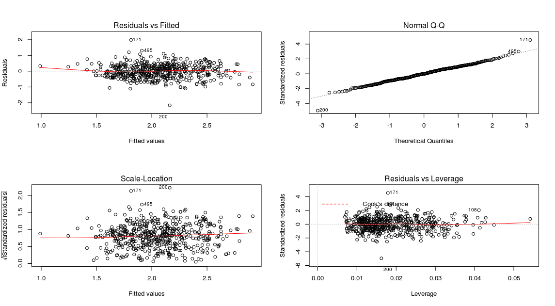
Thus, the diagnostic plot is also look fair. So, possibly the multicollinearity problem is the reason for not getting many insignificant regression coefficients.
For further diagnosis of the problem, let us first look at the pair-wise correlation among the explanatory variables.
X<-wagesmicrodata[,3:12]
library(GGally)
ggpairs(X)
Gives this plot:
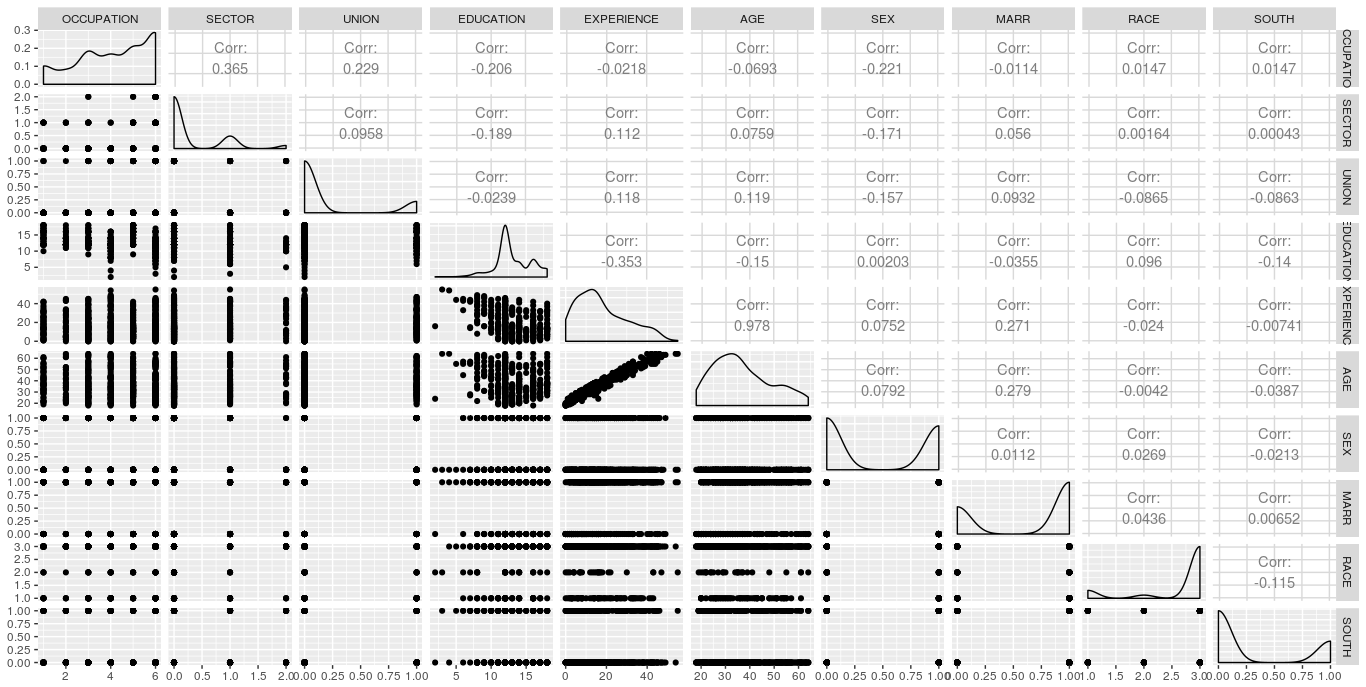
The correlation matrix shows that the pair-wise correlation among all the explanatory variables are not very high, except for the pair age – experience. The high correlation between age and experience might be the root cause of multicollinearity.
Again by looking at the partial correlation coefficient matrix among the variables, it is also clear that the partial correlation between experience – education, age – education and age – experience are quite high.
library(corpcor)
cor2pcor(cov(X))
             [,1]         [,2]         [,3]         [,4]        [,5]        [,6]         [,7]         [,8]         [,9]        [,10]
 [1,]  1.000000000  0.314746868  0.212996388  0.029436911  0.04205856 -0.04414029 -0.142750864 -0.018580965  0.057539374  0.008430595
 [2,]  0.314746868  1.000000000 -0.013531482 -0.021253493 -0.01326166  0.01456575 -0.112146760  0.036495494  0.006412099 -0.021518760
 [3,]  0.212996388 -0.013531482  1.000000000 -0.007479144 -0.01024445  0.01223890 -0.120087577  0.068918496 -0.107706183 -0.097548621
 [4,]  0.029436911 -0.021253493 -0.007479144  1.000000000 -0.99756187  0.99726160  0.051510483 -0.040302967  0.017230877 -0.031750193
 [5,]  0.042058560 -0.013261665 -0.010244447 -0.997561873  1.00000000  0.99987574  0.054977034 -0.040976643  0.010888486 -0.022313605
 [6,] -0.044140293  0.014565751  0.012238897  0.997261601  0.99987574  1.00000000 -0.053697851  0.045090327 -0.010803310  0.021525073
 [7,] -0.142750864 -0.112146760 -0.120087577  0.051510483  0.05497703 -0.05369785  1.000000000  0.004163264  0.020017315 -0.030152499
 [8,] -0.018580965  0.036495494  0.068918496 -0.040302967 -0.04097664  0.04509033  0.004163264  1.000000000  0.055645964  0.030418218
 [9,]  0.057539374  0.006412099 -0.107706183  0.017230877  0.01088849 -0.01080331  0.020017315  0.055645964  1.000000000 -0.111197596
[10,]  0.008430595 -0.021518760 -0.097548621 -0.031750193 -0.02231360  0.02152507 -0.030152499  0.030418218 -0.111197596  1.000000000
Farrar – Glauber Test
The ‘mctest’ package in R provides the Farrar-Glauber test and other relevant tests for multicollinearity. There are two functions viz. ‘omcdiag’ and ‘imcdiag’ under ‘mctest’ package in R which will provide the overall and individual diagnostic checking for multicollinearity respectively.
library(mctest)
omcdiag(X,WAGE)
Call:
omcdiag(x = X, y = WAGE)


Overall Multicollinearity Diagnostics

                       MC Results detection
Determinant |X'X|:         0.0001         1
Farrar Chi-Square:      4833.5751         1
Red Indicator:             0.1983         0
Sum of Lambda Inverse: 10068.8439         1
Theil's Method:            1.2263         1
Condition Number:        739.7337         1

1 --> COLLINEARITY is detected
0 --> COLLINEARITY in not detected by the test

===================================
Eigvenvalues with INTERCEPT
                   Intercept OCCUPATION SECTOR  UNION EDUCATION EXPERIENCE    AGE    SEX    MARR
Eigenvalues:          7.4264     0.9516 0.7635 0.6662    0.4205     0.3504 0.2672 0.0976  0.0462
Condition Indeces:    1.0000     2.7936 3.1187 3.3387    4.2027     4.6035 5.2719 8.7221 12.6725
                      RACE    SOUTH
Eigenvalues:        0.0103   0.0000
Condition Indeces: 26.8072 739.7337
The value of the standardized determinant is found to be 0.0001 which is very small. The calculated value of the Chi-square test statistic is found to be 4833.5751 and it is highly significant thereby implying the presence of multicollinearity in the model specification.
This induces us to go for the next step of Farrar – Glauber test (F – test) for the location of the multicollinearity.
imcdiag(X,WAGE)
Call:
imcdiag(x = X, y = WAGE)


All Individual Multicollinearity Diagnostics Result

                 VIF    TOL          Wi          Fi Leamer      CVIF Klein
OCCUPATION    1.2982 0.7703     17.3637     19.5715 0.8777    1.3279     0
SECTOR        1.1987 0.8343     11.5670     13.0378 0.9134    1.2260     0
UNION         1.1209 0.8922      7.0368      7.9315 0.9445    1.1464     0
EDUCATION   231.1956 0.0043  13402.4982  15106.5849 0.0658  236.4725     1
EXPERIENCE 5184.0939 0.0002 301771.2445 340140.5368 0.0139 5302.4188     1
AGE        4645.6650 0.0002 270422.7164 304806.1391 0.0147 4751.7005     1
SEX           1.0916 0.9161      5.3351      6.0135 0.9571    1.1165     0
MARR          1.0961 0.9123      5.5969      6.3085 0.9551    1.1211     0
RACE          1.0371 0.9642      2.1622      2.4372 0.9819    1.0608     0
SOUTH         1.0468 0.9553      2.7264      3.0731 0.9774    1.0707     0

1 --> COLLINEARITY is detected
0 --> COLLINEARITY in not detected by the test

OCCUPATION , SECTOR , EDUCATION , EXPERIENCE , AGE , MARR , RACE , SOUTH , coefficient(s) are non-significant may be due to multicollinearity

R-square of y on all x: 0.2805

* use method argument to check which regressors may be the reason of collinearity
===================================
The VIF, TOL and Wi columns provide the diagnostic output for variance inflation factor, tolerance and Farrar-Glauber F-test respectively. The F-statistic for the variable ‘experience’ is quite high (5184.0939) followed by the variable ‘age’ (F -value of 4645.6650) and ‘education’ (F-value of 231.1956). The degrees of freedom is \( (k-1 , n-k) \)or (9, 524). For this degrees of freedom at 5% level of significance, the theoretical value of F is 1.89774. Thus, the F test shows that either the variable ‘experience’ or ‘age’ or ‘education’ will be the root cause of multicollinearity. Though the F -value for ‘education’ is also significant, it may happen due to inclusion of highly collinear variables such as ‘age’ and ‘experience’.
Finally, for examining the pattern of multicollinearity, it is required to conduct t-test for correlation coefficient. As there are ten explanatory variables, there will be six pairs of partial correlation coefficients. In R, there are several packages for getting the partial correlation coefficients along with the t- test for checking their significance level. We’ll the ‘ppcor’ package to compute the partial correlation coefficients along with the t-statistic and corresponding p-values.
library(ppcor)
pcor(X, method = "pearson")
$estimate
             OCCUPATION       SECTOR        UNION    EDUCATION  EXPERIENCE         AGE          SEX         MARR         RACE        SOUTH
OCCUPATION  1.000000000  0.314746868  0.212996388  0.029436911  0.04205856 -0.04414029 -0.142750864 -0.018580965  0.057539374  0.008430595
SECTOR      0.314746868  1.000000000 -0.013531482 -0.021253493 -0.01326166  0.01456575 -0.112146760  0.036495494  0.006412099 -0.021518760
UNION       0.212996388 -0.013531482  1.000000000 -0.007479144 -0.01024445  0.01223890 -0.120087577  0.068918496 -0.107706183 -0.097548621
EDUCATION   0.029436911 -0.021253493 -0.007479144  1.000000000 -0.99756187  0.99726160  0.051510483 -0.040302967  0.017230877 -0.031750193
EXPERIENCE  0.042058560 -0.013261665 -0.010244447 -0.997561873  1.00000000  0.99987574  0.054977034 -0.040976643  0.010888486 -0.022313605
AGE        -0.044140293  0.014565751  0.012238897  0.997261601  0.99987574  1.00000000 -0.053697851  0.045090327 -0.010803310  0.021525073
SEX        -0.142750864 -0.112146760 -0.120087577  0.051510483  0.05497703 -0.05369785  1.000000000  0.004163264  0.020017315 -0.030152499
MARR       -0.018580965  0.036495494  0.068918496 -0.040302967 -0.04097664  0.04509033  0.004163264  1.000000000  0.055645964  0.030418218
RACE        0.057539374  0.006412099 -0.107706183  0.017230877  0.01088849 -0.01080331  0.020017315  0.055645964  1.000000000 -0.111197596
SOUTH       0.008430595 -0.021518760 -0.097548621 -0.031750193 -0.02231360  0.02152507 -0.030152499  0.030418218 -0.111197596  1.000000000

$p.value
             OCCUPATION       SECTOR        UNION EDUCATION EXPERIENCE       AGE         SEX      MARR       RACE      SOUTH
OCCUPATION 0.000000e+00 1.467261e-13 8.220095e-07 0.5005235  0.3356824 0.3122902 0.001027137 0.6707116 0.18763758 0.84704000
SECTOR     1.467261e-13 0.000000e+00 7.568528e-01 0.6267278  0.7615531 0.7389200 0.010051378 0.4035489 0.88336002 0.62243025
UNION      8.220095e-07 7.568528e-01 0.000000e+00 0.8641246  0.8146741 0.7794483 0.005822656 0.1143954 0.01345383 0.02526916
EDUCATION  5.005235e-01 6.267278e-01 8.641246e-01 0.0000000  0.0000000 0.0000000 0.238259049 0.3562616 0.69337880 0.46745162
EXPERIENCE 3.356824e-01 7.615531e-01 8.146741e-01 0.0000000  0.0000000 0.0000000 0.208090393 0.3482728 0.80325456 0.60962999
AGE        3.122902e-01 7.389200e-01 7.794483e-01 0.0000000  0.0000000 0.0000000 0.218884070 0.3019796 0.80476248 0.62232811
SEX        1.027137e-03 1.005138e-02 5.822656e-03 0.2382590  0.2080904 0.2188841 0.000000000 0.9241112 0.64692038 0.49016279
MARR       6.707116e-01 4.035489e-01 1.143954e-01 0.3562616  0.3482728 0.3019796 0.924111163 0.0000000 0.20260170 0.48634504
RACE       1.876376e-01 8.833600e-01 1.345383e-02 0.6933788  0.8032546 0.8047625 0.646920379 0.2026017 0.00000000 0.01070652
SOUTH      8.470400e-01 6.224302e-01 2.526916e-02 0.4674516  0.6096300 0.6223281 0.490162786 0.4863450 0.01070652 0.00000000

$statistic
           OCCUPATION     SECTOR      UNION    EDUCATION   EXPERIENCE          AGE         SEX        MARR       RACE      SOUTH
OCCUPATION  0.0000000  7.5906763  4.9902208    0.6741338    0.9636171   -1.0114033 -3.30152873 -0.42541117  1.3193223  0.1929920
SECTOR      7.5906763  0.0000000 -0.3097781   -0.4866246   -0.3036001    0.3334607 -2.58345399  0.83597695  0.1467827 -0.4927010
UNION       4.9902208 -0.3097781  0.0000000   -0.1712102   -0.2345184    0.2801822 -2.76896848  1.58137652 -2.4799336 -2.2436907
EDUCATION   0.6741338 -0.4866246 -0.1712102    0.0000000 -327.2105031  308.6803174  1.18069629 -0.92332727  0.3944914 -0.7271618
EXPERIENCE  0.9636171 -0.3036001 -0.2345184 -327.2105031    0.0000000 1451.9092015  1.26038801 -0.93878671  0.2492636 -0.5109090
AGE        -1.0114033  0.3334607  0.2801822  308.6803174 1451.9092015    0.0000000 -1.23097601  1.03321563 -0.2473135  0.4928456
SEX        -3.3015287 -2.5834540 -2.7689685    1.1806963    1.2603880   -1.2309760  0.00000000  0.09530228  0.4583091 -0.6905362
MARR       -0.4254112  0.8359769  1.5813765   -0.9233273   -0.9387867    1.0332156  0.09530228  0.00000000  1.2757711  0.6966272
RACE        1.3193223  0.1467827 -2.4799336    0.3944914    0.2492636   -0.2473135  0.45830912  1.27577106  0.0000000 -2.5613138
SOUTH       0.1929920 -0.4927010 -2.2436907   -0.7271618   -0.5109090    0.4928456 -0.69053623  0.69662719 -2.5613138  0.0000000

$n
[1] 534

$gp
[1] 8

$method
[1] "pearson"
As expected the high partial correlation between ‘age’ and ‘experience’ is found to be highly statistically significant. Similar is the case for ‘education – experience’ and ‘education – age’ . Not only that even some of the low correlation coefficients are also found to be highyl significant. Thus, the Farrar-Glauber test points out that X1 is the root cause of all multicollinearity problem.
Remedial Measures
There are several remedial measure to deal with the problem of multicollinearity such Prinicipal Component Regression, Ridge Regression, Stepwise Regression etc.
However, in the present case, I’ll go for the exclusion of the variables for which the VIF values are above 10 and as well as the concerned variable logically seems to be redundant. Age and experience will certainly be correlated. So, why to use both of them? If we use ‘age’ or ‘age-squared’, it will reflect the experience of the respondent also. Thus, we try to build a model by excluding ‘experience’, estimate the model and go for further diagnosis for the presence of multicollinearity.
fit2<- lm(log(WAGE)~OCCUPATION+SECTOR+UNION+EDUCATION+AGE+SEX+MARR+RACE+SOUTH)
summary(fit3)
Call:
lm(formula = log(WAGE) ~ OCCUPATION + SECTOR + UNION + EDUCATION +
    AGE + SEX + MARR + RACE + SOUTH)

Residuals:
     Min       1Q   Median       3Q      Max
-2.16018 -0.29085 -0.00513  0.29985  1.97932

Coefficients:
             Estimate Std. Error t value Pr(>|t|)
(Intercept)  0.501358   0.164794   3.042 0.002465 **
OCCUPATION  -0.006941   0.013095  -0.530 0.596309
SECTOR       0.091013   0.038723   2.350 0.019125 *
UNION        0.200018   0.052459   3.813 0.000154 ***
EDUCATION    0.083815   0.007728  10.846  < 2e-16 ***
AGE          0.010305   0.001745   5.905 6.34e-09 ***
SEX         -0.220100   0.039837  -5.525 5.20e-08 ***
MARR         0.075125   0.041886   1.794 0.073458 .
RACE         0.050674   0.028523   1.777 0.076210 .
SOUTH       -0.103186   0.042802  -2.411 0.016261 *
---
Signif. codes:  0 ‘***’ 0.001 ‘**’ 0.01 ‘*’ 0.05 ‘.’ 0.1 ‘ ’ 1

Residual standard error: 0.4397 on 524 degrees of freedom
Multiple R-squared:  0.3175,    Adjusted R-squared:  0.3058
F-statistic: 27.09 on 9 and 524 DF,  p-value: < 2.2e-16
Now by looking at the significance level, it is seen that out of nine of regression coefficients, eight are statistically significant. The R-square value is 0.31 and F-value is also very high and significant too.
Even the VIF values for the explanatory variables have reduced to very lower values.
vif(fit2)
OCCUPATION     SECTOR      UNION  EDUCATION        AGE        SEX       MARR       RACE      SOUTH
  1.295935   1.198460   1.120743   1.125994   1.154496   1.088334   1.094289   1.037015 1.046306
So, the model is now free from multicollinearity.
BEWARE: This is a clear example of a miss use of linear regression. You are including categorical variables as if they were numerical in the model, this is a very common mistake with non statisticians using linear models. Just to prove my point, can you interpret the value associated with term occupation (-0.007417)? remember that this variable has the following codification: (1=Management, 2=Sales, 3=Clerical, 4=Service, 5=Professional, 6=Other).
Before fitting the model, you should run this chunk first:
for(i in c("SOUTH","SEX","UNION","RACE","OCCUPATION","SECTOR","MARR")){wagesmicrodata[,i]<-factor(wagesmicrodata[,i]) }
Dear Nicolas, you are correct. I have used to the categorical variables simply treating them numerical just to demonstrate the multicollinearity problem. You can simply tweak the codes to treate them categorical by using as.factor function in R. My intention was not in finding the actual relationship among the variables; rather to demonstrate the codes/functions to find out the multicollinearity model simply ignoring the categorical variables. For actual research works, obviuously we need to take care of all. If you add so many categorical variables using dummy variables, then interpretation will become complex and the main focal point will not covered. By the way i am from statistical background only.
Am liking this already, let me continue reading
two (marital status and south) are significant only at 10 % level of significance – Is this statement accurate?
Best of the best!
Great Job
Very explanative! Thank you.
welcome
So Farrar – Glauber Test can be used to check multicollinearity for both numerical and categorical independent variables ?
Could you clarify me please?
I could not understand the meaning of numerical variable exactly. Probably you want to mean the ratio scale variable. If it is so, my answer is ‘yes’. The test is applicable
Hi Bidyut,
Thanks for the detailed explanation.
I have a quick question, Sometimes lm() summary shows coefficients for individual values in the columns and within that some column values are statistically significant for the model. Sometimes those coming with NA in coefficients summary.
Your thoughts here would be benificial for me.
Regards,
Nantha.
In R, NA stands for ‘Not Available’
Well done! Thank You
You are most welcom
You are most welcome
good work!
It is so far the best article I have read on multicollinearity. It integrates theory and practice.
I have been thinking of writing such an article on this topic, but as long as we have this article, there is no need for that.
Excellent work!
Thank you
Welcome
Amazing article and very informational. Loved reading it.
Thank you…..Anishji
Very nice work. Thank you for this detailed post.
You are most welcome