In the last two posts, I’ve focused purely on statistical topics – one-way ANOVA and dealing with multicollinearity in R. In this post, I’ll deviate from the pure statistical topics and will try to highlight some aspects of qualitative research. More specifically, I’ll show you the procedure of analyzing text mining and visualizing the text analysis using word cloud.
Some of typical usage of the text mining are mentioned below:
- – Marketing managers often use the text mining approach to study the needs and complaints of their customers;
– Politicians and journalists also use effectively the text mining to critically analyze the lectures delivered by the opposition leaders;
– Social media experts uses this technique to collect, analyze and share user posts, comments etc.;
– Social science researchers use text mining approach for analysing the qualitative data.
What is Text mining?
It is method which enables us to highlight the most frequently used keywords in a paragraph of texts or compilation of several text documents.
What is Word Cloud?
It is the visual representation of text data, especially the keywords in the text documents.
R has very simple and straightforward approaches for text mining and creating word clouds.
The text mining package “(tm)” will be used for mining the text and the word cloud generator package (wordcloud) will be used for visualizing the keywords as a word cloud.
Preparing the Text Documents:
As the starting point of qualitative research, you need to create the text file. Here I’ve used the lecture delivered by great Indian Hindu monk Swami Vivekananda at the first World’s Parliament of Religions held from 11 to 27 September 1893. Only two lecture notes – opening and closing address, will be used.
Both the lectures are saved in text file (chicago).
Loading the Required Packages:
library("tm")
library("SnowballC")
library("wordcloud")
library("RColorBrewer")
Load the text:
Importing the text file:
The text file (chicago) is imported using the following code in R.
The R code for leading the text is given below:
text <- readLines(file.choose())
Build the data as a corpus:
The ‘text’ object will now be loaded as ‘Corpora’ which are collections of documents containing (natural language) text. The Corpus() function from text mining(tm) package will be used for this purpose.
The R code for building the corpus is given below:
docs <- Corpus(VectorSource(text))
Next use the function inspect() under the tm package to display detailed information of the text document.
The R code for inspecting the text is given below:
inspect(docs)
The output is not, however, produced here due to space constraint
Text transformation:
After inspecting the text document (corpora), it is required to perform some text transformation for replacing special characters from the text. To do this, use the ‘tm_map()’ function.
The R code for transformation of the text is given below:
toSpace <- content_transformer(function (x , pattern ) gsub(pattern, " ", x))
docs <- tm_map(docs, toSpace, "/")
docs <- tm_map(docs, toSpace, "@")
docs <- tm_map(docs, toSpace, "\\|")
Text Cleaning:
After removing the special characters from the text, it is now the time to remove the to remove unnecessary white space, to convert the text to lower case, to remove common stopwords like ‘the’, “we”. This is required as the The information value of ‘stopwords’ is near zero due to the fact that they are so common in a language. For doing this exercise, the same ‘tm_map()’ function will be used.
The R code for cleaning the text along with the short self-explanation is given below:
# Convert the text to lower case
docs <- tm_map(docs, content_transformer(tolower))
# Remove numbers
docs <- tm_map(docs, removeNumbers)
# Remove english common stopwords
docs <- tm_map(docs, removeWords, stopwords("english"))
# Remove your own stop word
# specify your stopwords as a character vector
docs <- tm_map(docs, removeWords, c("I", "my"))
# Remove punctuations
docs <- tm_map(docs, removePunctuation)
# Eliminate extra white spaces
docs <- tm_map(docs, stripWhitespace)
Building a document matrix:
Document matrix is the frequency distribution of the words used in the given text. I hope that readers will easily understand this frequency distribution of words.
The R function TermDocumentMatrix() from the text mining package ‘tm’ will be used for building this frequency table for words in the given text.
The R code is given below:
docs_matrix <- TermDocumentMatrix(docs)
m <- as.matrix(docs_matrix)
v <- sort(rowSums(m),decreasing=TRUE)
d <- data.frame(word = names(v),freq=v)
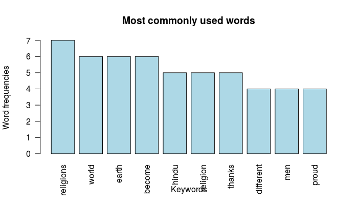
Have a look at the document matrix for the top ten keywords:
head(d, 10)
               word freq
religions religions    7
world         world    6
earth         earth    6
become       become    6
hindu         hindu    5
religion   religion    5
thanks       thanks    5
different different    4
men             men    4
proud         proud    4
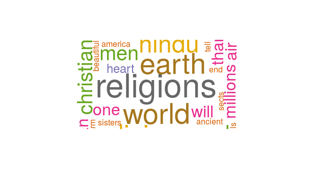
Generate the Word cloud:
Finally, the frequency table of the words (document matrix) will be visualized graphically by plotting in a word cloud with the help of the following R code.
wordcloud(words = d$word, freq = d$freq, min.freq = 1,
          max.words=200, random.order=FALSE, rot.per=0.35,
          colors=brewer.pal(8, "Dark2"))
You can also use barplot to plot the frequencies of the keywords using the following R code:
barplot(d[1:10,]$freq, las = 2, names.arg = d[1:10,]$word,
        col ="lightblue", main ="Most commonly used words",
        ylab = "Word frequencies", xlab="Keywords")
Conclusion:
The above word cloud clearly shows that “religions”, “earth”, “world”, “hindu”, “one” etc. are the most important words in the lecture delivered by Swamiji in Chicago World’s Parliament of Religions.