Welcome to Part 3 of my series on “Visualizing the World Cup with R”! This is the culmination of this mini project that I've been working on throughout the World Cup (You can check out the Github Repo here). In addition, from having listened to Thomas Pedersen's excellent keynote at UseR! 2018 in Brisbane on the NEW gganimate and tweenr API, I am taking advantage of the fortuitous timing to also compare the APIs using the goals as the examples!
I've had finished these animations a couple of weeks ago but didn't make them available until I presented at the TokyoR MeetUp last week! Hadley Wickham and Joe Rickert were the special guests and with the amount of speakers and attendees it felt more like a mini-conference than a regular meetup, if you're ever in Tokyo come join us for some R&R…and R! You can check out a recording of my talk on YouTube.
Let's get started!
Coordinate position data
Since this series started, several people have asked me where I got the data. I thought I made it quite clear in Part 1 but I will reiterate in the next few paragraphs.
I get a lot of my data science/visualization news from Twitter which has made a weird comeback by providing a platform for certain communities like #rstats (never thought I'll be creating a Twitter account in 2017!). Therefore, I've been able to come across some wonderful visualizations for the World Cup by The Financial Times, FiveThirtyEight, and a host of other people. As you can see from a great example of World Cup penalties by the BBC below, data is provided by sports analytics companies, primarily Opta!
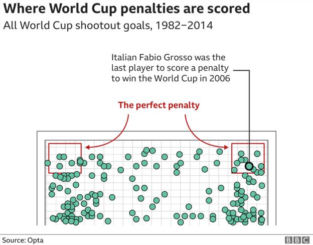
Great! But can an average joe like me just waltz in, slap down a fiver, and say “GIMME THE DATA”? Well, unfortunately no, it costs quite a lot! This isn't really a knock on Opta or other sports analytics companies since FIFA or the FAs of respective nations didn't do this kind of stuff, the free market stepped in to fill the gap. Still, I'm 100% sure I am not the only one who wishes this kind of data was free though, well besides some datasets of varying quality you see on Kaggle (but none of those are as granular as the stuff Opta provides anyway).
So, envious of those who have the financial backing to procure such data and some mild annoyance at others online who didn't really bother sharing exactly how they got their data or even what tools they used, I started thinking of ways that I could get the data for myself.
One possible way was to use RSelenium or other JavaScript web scrapers on soccer analytics websites and their cool dashboards, like WhoScored.com. However, since I wouldn't have been able to master these tools before the World Cup ended (during which whatever I end up creating would be most relevant), I decided that I'll create the coordinate data positions myself!
With the plotting system in ggsoccer and ggplot2 it's really not that hard to figure out the positions on the soccer field plot, as you can see in the picture below:
ggplot(point_data) +
  annotate_pitch() +
  theme_pitch(aspect_ratio = NULL) +
  coord_flip() +
  geom_point(
    aes(x = x, y = y),
    size = 1.5) +
  geom_text(
    aes(x = x, y = y,
        label = label),
    vjust = 1.5, color = "red")
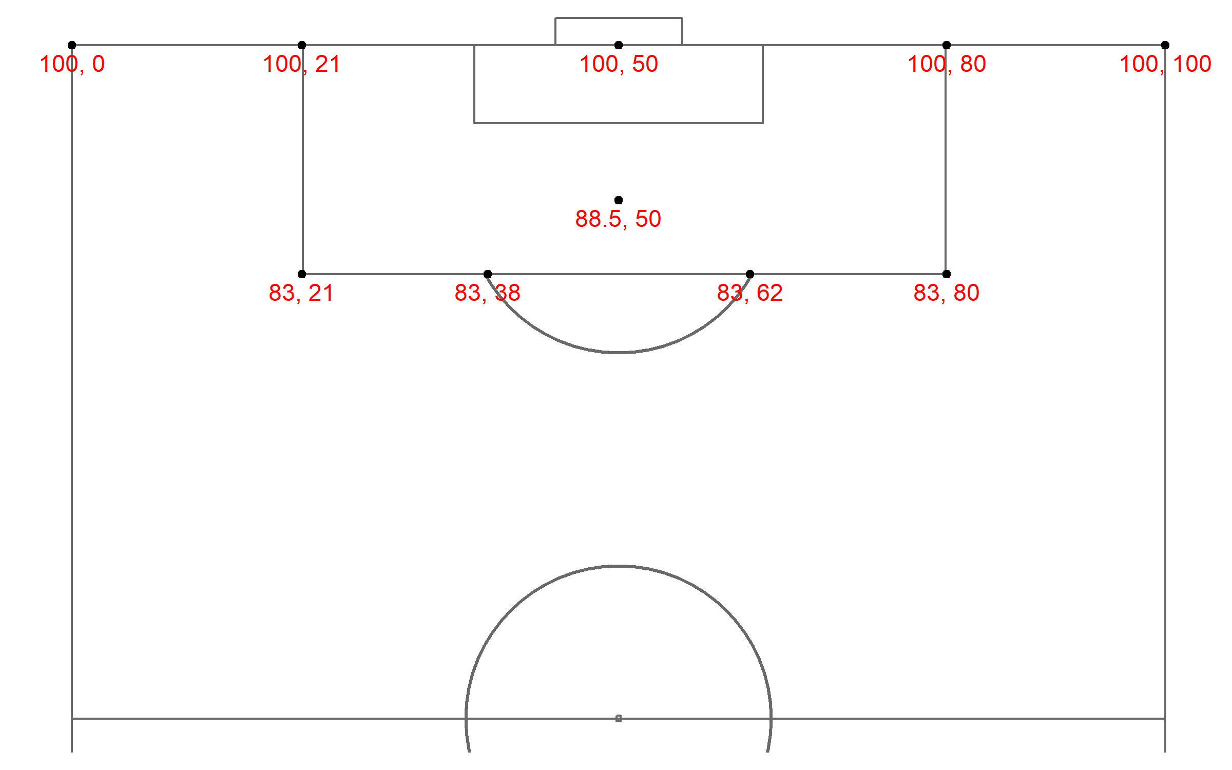
There's also a way to make the coordinates be in 120×80 format (which is much more intuitive) and you can do that by adding the *_scale arguments inside the annotate_pitch() function. However, I only realized this after I had embedded the coordinate positions for the 100×100 plot in my head so that's what I kept going with.
There is also the “Soccer event logger” here (incidentally also by Ben Torvaney) which allows you to mouse-click specific points on the field and then download a .csv file of the coordinate positions you clicked. This might be easier but personally, I like to experiment within the R environment and take notes/ideas in RMarkdown as I do so, it definitely is an option for others though.
… and that's how Part 1 was born! But I wasn't going to stop there, soccer is a moving – flowing game, static images are OK but it just doesn't capture the FEEL of the sport. So this is where gganimate and tweenr came in!
Out of all the World Cup stuff I've animated so far, by far the most complicated was Gazinsky's goal in the opening game. This is because I not only have to track the ball movement but the movement of multiple players as well. So most of the comparison aspect of the APIs will be done with this goal.
Let's take a look at the packages that I'll be using:
library(ggplot2)    # general plotting base
library(dplyr)      # data manipulation/tidying
library(ggsoccer)   # draw soccer field plot
library(ggimage)    # add soccer ball emoji + flags
library(extrafont)  # incorporate Dusha font into plots
library(gganimate)  # animate goal plots
library(tweenr)     # create in-between frames for data
library(purrr)      # for creating a list of dataframes for tweenr
library(countrycode)# for finding ISO codes for geom_flag()
# loadfonts()         run once every new session
Gazinsky's first goal
Let's first look at the set of dataframes with the coordinate data points necessary for this to work:
pass_data <- data.frame(
  x = c(100, 94, 82, 82.5,  84, 76.5, 75.5, 94, 99.2),
  y = c(0,   35, 31, 22,     8, 13, 19, 60, 47.5),
  time = c(1, 2, 3, 4, 5, 6, 7, 8, 9))

golovin_movement <- data.frame(
  x = c(78, 80, 80, 80, 75.5, 74.5, 73.5, 73, 73),
  y = c(30, 30, 27, 25,   10,    9, 15, 15, 15),
  label = "Golovin",
  time = c(1, 2, 3,  4,  5,  6,  7,  8,  9)
)

zhirkov_movement <- data.frame(
  x = c(98, 90, 84, 84, 84, 84, 84, 84, 84),
  y = c( 0,  2,  2,  2,  2,  2,  2,  2,  2),
  label = "Zhirkov",
  time = c(1, 2, 3, 4, 5, 6, 7, 8, 9)
)

gazinsky_movement <- data.frame(
  x = c(0, 0, 0, 0, NA, 92,   92,   92,   92),
  y = c(0, 0, 0, 0, NA, 66.8, 66.8, 66.8, 66.8),
  label = "Gazinsky",
  time = c(1, 2, 3, 4, 5, 6, 7, 8, 9)
)

# ONLY in static + gganimate versions
segment_data <- data.frame(
  x = c(77.5, 98),
  y = c(22, 2),
  xend = c(75, 84),
  yend = c(15, 3),
  linetype = c("dashed", "dashed"),
  color = c("black", "black"),
  size = c(1.2, 1.25)
)

# saudi defender
saudi_data <- data.frame(
  x = c(95, 95, 90, 87, 84, 80, 79, 79, 79),
  y = c(35, 35, 35, 32, 28, 25, 24, 25, 26),
  label = "M. Al-Breik",
  time = c(1, 2, 3, 4, 5, 6, 7, 8, 9)
)

### soccer ball
ball_data <- tribble(
  ~x,  ~y, ~time,
  100,   0,   1,
  94,   35,   2,
  82,   31,   3,
  82.5, 25,   4,
  84,    6,   5,
  77,   13,   6,
  76,   19,   7,
  94,   60,   8,
  99.2, 47.5, 9

)
If you're manually creating these, you could also use tribble() instead of a dataframe(). It takes up a bit more space, as you can see in ball_data, but it is probably more readable for when you're sharing the code (like creating a reprex on SO or RStudio Community).
And here is the ggplot code for the gganimate version (no tween frames)!
Note: You need to be careful about the ordering of the ggplot elements. You need to make sure the soccer ball emoji code is near the end, after the labels, so that the player name labels don't cover the soccer ball as it's moving around!
ggplot(pass_data) +
  annotate_pitch() +
  theme_pitch() +
  coord_flip(
    xlim = c(49, 101),
    ylim = c(-1, 101)) +
  geom_segment(
    data = segment_data,
    aes(x = x, y = y,
        xend = xend, yend = yend),
    size = segment_data$size,
    color = segment_data$color,
    linetype = c("dashed", "dashed")) +
  geom_label(
    data = saudi_data,
    aes(x = x, y = y,
        label = label),
    color = "darkgreen") +
  geom_label(data = zhirkov_movement,
    aes(x = x, y = y,
        frame = time,
        label = label),
    color = "red") +
  geom_label(data = golovin_movement,
    aes(x = x, y = y,
        frame = time,
        label = label),
    color = "red") +
  geom_label(
    data = gazinsky_movement,
    aes(x = x, y = y,
        label = label),
    color = "red") +
  ggimage::geom_emoji(
    data = ball_data,
    aes(x = x, y = y, frame = time),
    image = "26bd", size = 0.035) +
  ggtitle(
    label = "Russia (5) vs. (0) Saudi Arabia",
    subtitle = "First goal, Yuri Gazinsky (12th Minute)") +
  labs(caption = "By Ryo Nakagawara (@R_by_Ryo)") +
  annotate(
    "text", x = 69, y = 65, family = "Dusha V5",
    label = "After a poor corner kick clearance\n from Saudi Arabia, Golovin picks up the loose ball, \n exchanges a give-and-go pass with Zhirkov\n before finding Gazinsky with a beautiful cross!") +
  theme(text = element_text(family = "Dusha V5"))
Now let's check out how we would do it with the in-between frames added in using tweenr!
The important bit with the old API was that you had to create a list of dataframes of the different states of your data. In this case, it is a dataframe for each observation of the data or to put it more simply, the “time” variable (a dataframe of coordinate positions for time = 1, time = 2, etc.). This is done with pmap() with dataframe() being passed to the .f argument.
With this list of dataframes created, we can pass it into tween_states() function to create the in-between frames to connect each of the dataframes in the list. Take note of the arguments in tweent_states() as they'll show up again in the new API later.
### soccer ball
b_list <- ball_data %>% pmap(data.frame)

ball_tween <- b_list %>%
  tween_states(tweenlength = 0.5, statelength = 0.00000001, ease = "linear", nframes = 75)

### Golovin
golovin_movement_list <- golovin_movement %>% pmap(data.frame)

golovin_tween <- golovin_movement_list %>%
  tween_states(tweenlength = 0.5, statelength = 0.00000001, ease = "linear", nframes = 75)

golovin_tween <- golovin_tween %>% mutate(label = "Golovin")

### Zhirkov
zhirkov_movement_list <- zhirkov_movement %>% pmap(data.frame)

zhirkov_tween <- zhirkov_movement_list %>%
  tween_states(tweenlength = 0.5, statelength = 0.00000001, ease = "linear", nframes = 75)

zhirkov_tween <- zhirkov_tween %>% mutate(label = "Zhirkov")
Now with these newly created tween dataframes, we pass them into our ggplot code as before and specify the frame argument with the newly created “.frame” variable.
ggplot(pass_data) +
  annotate_pitch() +
  theme_pitch() +
  coord_flip(xlim = c(49, 101),
             ylim = c(-1, 101)) +
  geom_label(
    data = saudi_data,
    aes(x = x, y = y,
        label = label),
    color = "darkgreen") +
  geom_label(data = zhirkov_tween,
    aes(x = x, y = y,
        frame = .frame,
        label = label),
    color = "red") +
  geom_label(data = golovin_tween,
    aes(x = x, y = y,
        frame = .frame,
        label = label),
    color = "red") +
  geom_label(
    data = gazinsky_movement,
    aes(x = x, y = y,
        label = label),
    color = "red") +
  ggimage::geom_emoji(
    data = ball_tween,
    aes(x = x, y = y, frame = .frame),
    image = "26bd", size = 0.035) +
  ggtitle(label = "Russia (5) vs. (0) Saudi Arabia",
          subtitle = "First goal, Yuri Gazinsky (12th Minute)") +
  labs(caption = "By Ryo Nakagawara (@R_by_Ryo)") +
  annotate("text", x = 69, y = 65, family = "Dusha V5",
           label = "After a poor corner kick clearance\n from Saudi Arabia, Golovin picks up the loose ball, \n exchanges a give-and-go pass with Zhirkov\n before finding Gazinsky with a beautiful cross!") +
  theme(text = element_text(family = "Dusha V5"))
Looks good. Now, let's check out how things changed with the new API!
New gganimate & tweenr
Once again, let's start by looking at just animating across the “time” variable without creating in-between frames.
ggplot(pass_data) +
  annotate_pitch() +
  theme_pitch() +
  theme(text = element_text(family = "Dusha V5")) +
  coord_flip(xlim = c(49, 101),
             ylim = c(-1, 101)) +
  geom_label(
    data = zhirkov_movement,
    aes(x = x, y = y,
        label = label),
    color = "red") +
  geom_label(
    data = golovin_movement,
    aes(x = x, y = y,
        label = label),
    color = "red") +
  geom_label(
    data = gazinsky_movement,
    aes(x = x, y = y,
        label = label),
    color = "red") +
  geom_label(
    data = saudi_data,
    aes(x = x, y = y,
        label = label),
    color = "darkgreen") +
  ggimage::geom_emoji(
    data = ball_data,
    aes(x = x, y = y),
    image = "26bd", size = 0.035) +
  ggtitle(label = "Russia (5) vs. (0) Saudi Arabia",
          subtitle = "First goal, Yuri Gazinsky (12th Minute)") +
  labs(caption = "By Ryo Nakagawara (@R_by_Ryo)") +
  annotate("text", x = 69, y = 65, family = "Dusha V5",
           label = "After a poor corner kick clearance\n from Saudi Arabia, Golovin picks up the loose ball, \n exchanges a give-and-go pass with Zhirkov\n before finding Gazinsky with a beautiful cross!") +
  # new gganimate code:
  transition_manual(frames = time)
It's quite nice that I don't have to specify frame = some_time_variable in every geom that I want animated now!
However, you can see that like in the old gganimate code the new transition_manual() function just speeds through the specified “time” variable without actually creating in-between frames. Let's use the other transition_*() functions to specify the tween frames and set the animation speed.
Here I will use transition_states() with “time” being the column I pass to the states argument. Instead of having to create a “.frame” column with the tween_states() function I can just pass the “time” variable into the transition_states() function and it will tween the frames for you in addition to the ggplot code! The transition_length argument is the same as the tween_length argument from the old tween_states() function and state_length argument is the same here too.
Unlike in the version I showed in my presentation, I added Mohammed Al-Breik's movement as well. I felt it was a bit silly (and unfair) to show him just standing there after his headed clearance!
ggplot(pass_data) +
  annotate_pitch() +
  theme_pitch() +
  coord_flip(xlim = c(49, 101),
             ylim = c(-1, 101)) +
  geom_label(
    data = saudi_data,
    aes(x = x, y = y,
        label = label),
    color = "darkgreen") +
  geom_label(
    data = zhirkov_movement,
    aes(x = x, y = y,
        label = label),
    color = "red") +
  geom_label(
    data = golovin_movement,
    aes(x = x, y = y,
        label = label),
    color = "red") +
  geom_label(
    data = gazinsky_movement,
    aes(x = x, y = y,
        label = label),
    color = "red") +
  enter_grow(fade = TRUE) +
  ggimage::geom_emoji(
    data = ball_data,
    aes(x = x, y = y),
    image = "26bd", size = 0.035) +
  ggtitle(
    label = "Russia (5) vs. (0) Saudi Arabia",
    subtitle = "First goal, Yuri Gazinsky (12th Minute)") +
  labs(caption = "By Ryo Nakagawara (@R_by_Ryo)") +
  annotate(
    "text", x = 69, y = 65, family = "Dusha V5",
    label = "After a poor corner kick clearance\n from Saudi Arabia, Golovin picks up the loose ball, \n exchanges a give-and-go pass with Zhirkov\n before finding Gazinsky with a beautiful cross!") +
  theme(text = element_text(family = "Dusha V5")) +
  # new gganimate code:
  transition_states(
    time,
    transition_length = 0.5,
    state_length = 0.0001,
    wrap = FALSE) +
  ease_aes("linear")

anim_save(filename = "gazin_new_tweenr.gif")
Now you may be wondering why I didn't use the more logical choice, the transition_time() function here so let me explain.
I manually created the timing of the coordinate data so naturally, the transitions would be slightly off compared to real data. This goal animation was split into 9 “time” values for each important bit of the play that I thought would transition well when connected with eachother. Then I ran it through gganimate to see if it flowed well and once I was satisfied, I let tweenr fill in the blanks between each “time” value.
With the new API however, using transition_time() function wouldn't allow me to control transition length and state length like with transition_states()! Try running the code above with transition_time(time = time) instead and you'll see what I mean.
If I had real data and the proper timing values in the “time” column that seamlessly worked with the coordinate data points it would have then been appropriate to use transition_time(). Some examples of these kind of data sets include the gapminder data set used in the package README which used the “year” variable or the data set in the cool NBA animation by James Curley seen here that had very granular data recording the coordinate positions and the exact times.
A cool new thing that you can play around with in the new gganimate are the different enter/exit animations! However, I couldn't really get it to work for Gazinsky's label… In the mtcars example on the gganimate GitHub Repo, the boxplots disappeared when there was no data for the specific combination of variables but I can't seem to properly set up the Gazinsky label dataframe correctly to implement it.
Ideally, I want Gazinsky's label to only show up from time = 6 onwards. I tried filling the coordinate positions for time = 1 to time = 5 with NAs or 0s but it didn't seem trigger the effect … when I tried with “x = 0, y = 0” in time = 5, the player label zipped in from the bottom of the screen to the penalty box at time = 6 and it was unintentionally very funny!
Any help here will be greatly appreciated!
Osako's goal vs. Colombia
Japan faced a tough opponent in Colombia, even with the man-advantage early on, in our opening game of the World Cup. Even with our passing tiring out the tenacious Colombians we were finding it hard to find a breakthrough. In came Keisuke Honda, who within minutes of his arrival, delivered a beautiful cross from a corner kick for Osako to head home!
This goal was a lot easier to animate and to be honest this was the first one I was able to actually get working a few weeks ago! This was mainly because the ball movement was the only thing I really had to worry about.
cornerkick_data <- data.frame(
  x = 99, y = 0.3,
  x2 = 94, y2 = 47)

osako_gol <- data.frame(
  x = 94, y = 49,
  x2 = 100, y2 = 55.5)

ball_data <- data.frame(
  x = c(99, 94, 100),
  y = c(0.3, 47, 55.5),
  time = c(1, 2, 3))

player_label <- data.frame(
  x = c(92, 99),
  y = c(49, 2),
  label = c("Osako", "Honda"))

wc_logo <- data.frame(
  x = 107,
  y = 85) %>%
  mutate(
    image = "https://upload.wikimedia.org/wikipedia/en/thumb/6/67/2018_FIFA_World_Cup.svg/1200px-2018_FIFA_World_Cup.svg.png")

flag_data <- data.frame(
  x = c(110, 110),
  y = c( 13, 53),
  team = c("japan", "colombia")
  ) %>%
  mutate(
    image = team %>%
           countrycode(., origin = "country.name", destination = "iso2c")
  ) %>%
  select(-team)
For this animation, I used one of the many easing functions available in tweenr, quadratic-out, to get the speed of the ball from a corner kick just about right. You can refer to this awesome website to check out most of the different easing functions you can use in ease_aes()!
ggplot(ball_data) +
  annotate_pitch() +
  theme_pitch() +
  theme(
    text = element_text(family = "Dusha V5"),
    plot.margin=grid::unit(c(0,0,0,0), "mm")) +
  coord_flip(
    xlim = c(55, 112),
    ylim = c(-1, 101)) +
  geom_label(
    data = player_label,
    aes(x = x, y = y,
        label = label),
    family = "Dusha V5") +
  geom_point(
    aes(x = 98, y = 50), size = 3, color = "green") +
  annotate(
    geom = "text", family = "Dusha V5",
    hjust = c(0.5, 0.5, 0.5, 0.5),
    size = c(6.5, 4.5, 5, 3),
    label = c("Japan             (2) vs. Colombia             (1)",
              "Kagawa (PEN 6'), Quintero (39'), Osako (73')",
              "Japan press their man advantage, substitute Honda\ndelivers a delicious corner kick for Osako to (somehow) tower over\nColombia's defense and flick a header into the far corner!",
              "by Ryo Nakagawara (@R_by_Ryo)"),
    x = c(110, 105, 70, 53),
    y = c(30, 30, 47, 85)) +
  ggimage::geom_emoji(              # soccer ball emoji
    aes(x = x,
        y = y),
    image = "26bd", size = 0.035) +
  ggimage::geom_flag(               # Japan + Colombia flag
    data = flag_data,
    aes(x = x, y = y,
        image = image),
    size = c(0.08, 0.08)) +
  geom_image(                       # World Cup logo
    data = wc_logo,
    aes(x = x, y = y,
        image = image), size = 0.17) +
  # new gganimate code:
  transition_states(
    time,
    transition_length = 0.5,
    state_length = 0.0001,
    wrap = FALSE) +
  ease_aes("quadratic-out")
As you can see it's quite easy and fun to make these! I am hoping to make more in the future, especially when the new season begins!
A small note on the flags: I used a bit of a hacky solution to get them into the title but both Ben and Hadley recommended I use the emo::ji() package which allows you to insert emoji into RMarkdown and inline. So that's something I'll be looking into in the near future!
Japan's Offside Trap vs. Senegal!
For the final animation, I tried to recreate something you don't see everyday – an offside trap!
# PLAYERS
# JAPAN: x, y (blue)     Senegal: x2, y2  (lightgreen)
trap_data <- data.frame(

  time = c(1, 2, 3, 4, 5),

  # ball trajectory
  x = c(70, 70, 70, 87, 95),
  y = c(85, 85, 85, 52, 33),

  # offside line bar
  #xo =    c(83, 81.2, 79, 77.5, 70),
  xoend = c(83.8, 81.8, 79, 78.5, 71),

  yo =    c( 5,  5,  5,  5, 5),
  yoend = c(95, 95, 95, 95, 95),

  # players: japan
  jx  = c(83, 81, 77, 75, 70),
  jy  = c(rep(65, 5)),

  jx2 = c(83, 81.8, 78.5, 77, 70),
  jy2 = c(rep(60.5, 5)),

  jx3 = c(83, 81, 76.5, 75, 71),
  jy3 = c(rep(55, 5)),

  jx4 = c(83, 81.2, 76.3, 75, 70),
  jy4 = c(rep(52, 5)),

  jx5 = c(82.8, 81, 77, 74, 70),
  jy5 = c(rep(49, 5)),

  jx6 = c(83, 81.8, 77, 74, 70),
  jy6 = c(rep(45, 5)),

  jx7 = c(83.8, 81, 79, 77.5, 70),
  jy7 = c(rep(40, 5)),

  # players: senegal
  sx = c(83, 84, 84, 84, 84),
  sy = c(rep(33, 5)),

  sx2 = c(83, 85, 87, 92, 95),
  sy2 = c(38, 37, 35, 34, 33),

  sx3 = c(83, 84, 84, 83, 83),
  sy3 = c(rep(41, 5)),

  sx4 = c(83, 84, 83, 78, 78),
  sy4 = c(rep(45, 5)),

  sx5 = c(83, 84, 87, 88, 89),
  sy5 = c(rep(52, 5)),

  sx6 = c(83, 85, 84, 84, 83),
  sy6 = c(rep(69, 5))
)

# flags
flag_data <- data.frame(
  x = c( 48, 93),
  y = c(107, 107),
  team = c("japan", "senegal")
  ) %>%
  mutate(
    image = team %>%
           countrycode(., origin = "country.name", destination = "iso2c")
  ) %>%
  select(-team)

# extra players:
goalkeeper_data <- data.frame(
  x = c(98),
  y = c(50)
)

senegal_data <- data.frame(
  x = c(55, 55, 68.5),
  y = c(50, 60, 87)
)
In the code below, take note of the “wrap” option in transition_states(). You can set it to false if you don't want the last state to transition back to the first state (default == TRUE).
ggplot(trap_data) +
  annotate_pitch() +
  theme_pitch(aspect_ratio = NULL) +
  coord_fixed(
    xlim = c(30, 101),
    ylim = c(-5, 131)) +
  # offside line
  geom_segment(aes(x = xoend, y = yo,
                   xend = xoend, yend = yoend),
               color = "black", size = 1.3) +
  # japan
  geom_point(aes(x = jx, y = jy), size = 4, color = "blue") +
  geom_point(aes(x = jx2, y = jy2), size = 4, color = "blue") +
  geom_point(aes(x = jx3, y = jy3), size = 4, color = "blue") +
  geom_point(aes(x = jx4, y = jy4), size = 4, color = "blue") +
  geom_point(aes(x = jx5, y = jy5), size = 4, color = "blue") +
  geom_point(aes(x = jx6, y = jy6), size = 4, color = "blue") +
  geom_point(aes(x = jx7, y = jy7), size = 4, color = "blue") +
  # senegal
  geom_point(aes(x = sx, y = sy), size = 4, color = "green") +
  geom_point(aes(x = sx2, y = sy2), size = 4, color = "green") +
  geom_point(aes(x = sx3, y = sy3), size = 4, color = "green") +
  geom_point(aes(x = sx4, y = sy4), size = 4, color = "green") +
  geom_point(aes(x = sx5, y = sy5), size = 4, color = "green") +
  geom_point(aes(x = sx6, y = sy6), size = 4, color = "green") +

  # free kick spot (reference)
  geom_point(aes(x = 70, y = 85), color = "blue", size = 1.2) +
  # goalkeeper
  geom_point(
    data = goalkeeper_data,
    aes(x = x, y = y), size = 4, color = "blue") +
  # senegal defenders
  geom_point(
    data = senegal_data,
    aes(x = x, y = y), size = 4, color = "green") +
  annotate(
    geom = "text", family = "Dusha V5",
    hjust = c(0, 0),
    size = c(6, 6.5),
    label = c("Japan          (2) vs. Senegal         (2)",
              "The Perfect Offside Trap"),
    x = c(30,  30),
    y = c(107, 115)) +
  ggimage::geom_flag(
    data = flag_data,
    aes(x = x, y = y,
        image = image),
    size = c(0.07, 0.07)) +
  ggimage::geom_emoji(
    aes(x = x, y = y),
    image = "26bd", size = 0.035) +
  # NEW gganimate code
  transition_states(
    states = time,
    transition_length = 0.2,
    state_length = 0.00000001,
    wrap = FALSE) +
  ease_aes("linear")
Let's take a few minutes to reflect on the new API.
Personal thoughts
The best thing about the new API is without a doubt, no more intermediary steps between tweening the data and plotting. As long as you have some kind of “time” variable you don't have to manually go and create the list of data frame for each state yourself as transition_*() functions does it all for you in the ggplot code!
The ease_aes() also allows you to specify the easing function of the transitions within the ggplot code as well. From “linear” to “quartic” to “elastic” along with modifiers such as “in”, “out”, “in-out” you have a lot to choose from to satisfy your animation needs. Thomas did mention in his keynote that he wants a better name for this, so any suggestions? Maybe something like ease_tween(), easing_fun(), ease_trans(), ease_transitions()?
With everything streamlined so that you can add in the animation code seamlessly with ggplot grammar I feel you can read the entirety of the code better. As in, you don't have to refer back to a separate chunk of code that showed how you created the tween frames. The transition to a “grammar of animation” is truly in motion!
New options in gganimate and tweenr!
Now I'll talk about a few other new things that I didn't have a chance to show this time around.
There are a host of different enter_*() and exit_*() functions to choose from to show how data appear and disappear throughout the duration of your animation. Some of the built-in effects that are available include, *_fade(), *_grow(), *_shrink() with extra arguments like early that change whether the data appears or disappears at the beginning of the transition or at the end.
With the old API, since you had to create the frames yourself with tween_states(), you got a dataframe output with the expanded tween-frames that you could view at your leisure. Now with the tweening done in the ggplot code you might think that you can't explicitly access them, but this is where the frame_vars() function comes in! Using this function you can access metadata about each of the frames rendered in your latest animation:
frames_data <- frame_vars(animation = last_animation())
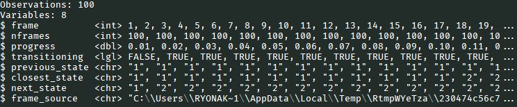
The “frame_source” column shows you where each individual frame image is saved so you can copy them, re-animate them with magick instead, anything you want!
Panning and zooming across different states in the animation is another new concept introduced in the new gganimate with the series of view_*() functions like view_zoom() and view_step(). Within these you can use arguments like pause_length to specify the length of the zoomed view and step_length to specify the length of the transition between view points. I didn't implement them in these GIFs because I had already used the coord_*() functions to focus on certain areas of the pitch and the events I was animating needed a wide perspective of the field. This may come into play in future goal or play-by-play animations where I'm recreating a neat bit of build-up play from a full field view then zoom in on the off-the-ball movement of a certain player, so definitely a set of functions to keep an eye on!
Finally, in previous versions you used the gganimate() function to save the animation on your computer but now that is done with anim_save(). The README on GitHub has a very clear explanation on this so take a look under the “Where is my animation?” section here.
There's still much to learn from the new API and I'm sure there will still be more changes/fixes to come before the first CRAN release but this was a great step in the right direction. I will eagerly await the next release!