This is the third post in our series Mastering R Plot, in this one we will cover the outer margins. To know more about plot customization read my first and second post.
Let’s directly dive into some code:
#a plot has inner and outer margins
#by default there is no outer margins
par()$oma
#but we can add some
op<-par(no.readonly=TRUE)
par(oma=c(2,2,2,2))
plot(1,1,type="n",xlab="",ylab="",xaxt="n",yaxt="n")
for(side in 1:4){
  inner<-round(par()$mar[side],0)-1
  for(line in 0:inner){
   mtext(text=paste0("Inner line ",line),side=side,line=line)
  }
  outer<-round(par()$oma[side],0)-1
   for(line in 0:inner){
   mtext(text=paste0("Outer line ",line),side=side,line=line,outer=TRUE)
  }
}
[1] 0 0 0 0
Here it is the plot:
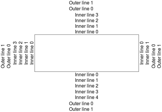
From this plot we see that we can control outer margins just like we controlled inner margins using the par function. To write text in the outer margins with the mtext function we need to set outer=TRUE in the function call.
Outer margins can be handy in various situations:
#Outer margins are useful in various context
#when axis label is long and one does not want to shrink plot area
par(op)
#example
par(cex.lab=1.7)
plot(1,1,ylab="A very very long axis title\nthat need special care",xlab="",type="n")
#one option would be to increase inner margin size
par(mar=c(5,7,4,2))
plot(1,1,ylab="A very very long axis title\nthat need special care",xlab="",type="n")
#sometime this is not desirable so one may plot the axis text outside of the plotting area
par(op)
par(oma=c(0,4,0,0))
plot(1,1,ylab="",xlab="",type="n")
mtext(text="A very very long axis title\nthat need special care",side=2,line=0,outer=TRUE,cex=1.7)
Here it is the plot:
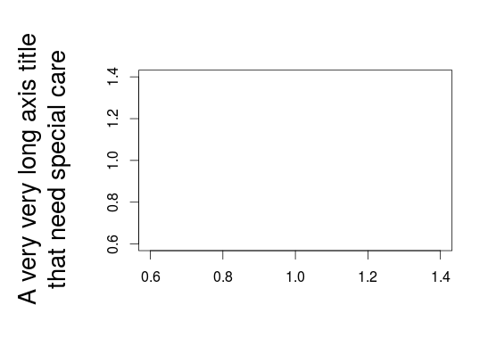
With outer margins we can write very long or very big axis labels or titles without having to “sacrifice” the size of the plotting region.
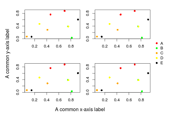
This comes especially handy for multi-panel plots:
#this is particularly useful when having a plot with multiple panels and similar axis labels
par(op)
par(oma=c(3,3,0,0),mar=c(3,3,2,2),mfrow=c(2,2))

plot(1,1,ylab="",xlab="",type="n")
plot(1,1,ylab="",xlab="",type="n")
plot(1,1,ylab="",xlab="",type="n")
plot(1,1,ylab="",xlab="",type="n")

mtext(text="A common x-axis label",side=1,line=0,outer=TRUE)
mtext(text="A common y-axis label",side=2,line=0,outer=TRUE)
Here it is the plot:

And we can also add a common legend:
set.seed(20160228)
#outer margins can also be used for plotting legend in them
x<-runif(10)
y<-runif(10)
cols<-rep(c("red","green","orange","yellow","black"),each=2)

par(op)
par(oma=c(2,2,0,4),mar=c(3,3,2,0),mfrow=c(2,2),pch=16)

for(i in 1:4){
  plot(x,y,col=cols,ylab="",xlab="")
}

mtext(text="A common x-axis label",side=1,line=0,outer=TRUE)
mtext(text="A common y-axis label",side=2,line=0,outer=TRUE)

legend(x=1,y=1.7,legend=LETTERS[1:5],col=unique(cols),pch=16,bty="n",xpd=NA)
Here it is the plot:
An important point to note here is that the xpd argument in the legend function which control if all plot elements (ie points, lines, legend, text …) are clipped to the plotting region if it is set to FALSE (the default value). If it is set to TRUE all plot elements are clipped to the figure region (plot + inner margins) and if it is set to NA you can basically add plot elements everywhere in the device region (plot + inner margins + outer margins). In the example above we set it to NA. Note that the xpd argument can also be set within the par function, it is then applied to all subsequent plots.
With all these tools in our hands we are now able to make our plots look just how we want them to. It is a matter of taste whether one prefer to use ggplot or plot to produce his/her final plots (I actually use them both) but I find that once one knows a bit about these funny arguments like cex, pch or oma it quickly gives what you want.
This was exactly what I needed. Thanks!
Nice summary. I’ll pass this on to grad students that I work with.
I’m partial to basic R graphics for its flexibility. I’ve found that it can do some things I’d spend much more time attempting in ggplot2. (See https://edwcarney.github.io/Basic-R-Graphics for some examples.)