In the present tutorial, we are going to analyze the mushroom dataset as made available by UCI Machine Learning (ref. [1]). This tutorial is structured as follows. First, we are going to gain some domain knowledge on mushrooms. That will help in understanding the dataset features. Then we will run an exploratory analysis. Afterwards, in the second part of this tutorial, we will build models to classify mushrooms as edible or poisoned. The R package and references lists shown ahead are about the overall tutorial.
Domain Knowledge
As anticipated, we are going to gain some basic domain knowledge about mushrooms.
Mushrooms Basics Concepts
A mushroom, or toadstool, is the fleshy, spore-bearing fruiting body of a fungus, typically produced above ground on soil or on its food source.
The standard for the name “mushroom” is the cultivated white button mushroom, Agaricus bisporus; hence the word “mushroom” is most often applied to those fungi (Basidiomycota, Agaricomycetes) that have a stem (stipe), a cap (pileus), and gills (lamellae, sing. lamella) on the underside of the cap. “Mushroom” also describes a variety of other gilled fungi, with or without stems, therefore the term is used to describe the fleshy fruiting bodies of some Ascomycota. These gills produce microscopic spores that help the fungus spread across the ground or its occupant surface.
Forms deviating from the standard morphology usually have more specific names, such as “bolete”, “puffball”, “stinkhorn”, and “morel”, and gilled mushrooms themselves are often called “agarics” in reference to their similarity to Agaricus or their order Agaricales. By extension, the term “mushroom” can also designate the entire fungus when in culture; the thallus (called a mycelium) of species forming the fruiting bodies called mushrooms; or the species itself.
Identifying mushrooms requires a basic understanding of their macroscopic structure. Most are Basidiomycetes and gilled. Their spores, called basidiospores, are produced on the gills and fall in a fine rain of powder from under the caps as a result. At the microscopic level the basidiospores are shot off basidia and then fall between the gills in the dead air space. As a result, for most mushrooms, if the cap is cut off and placed gill-side-down overnight, a powdery impression reflecting the shape of the gills (or pores, or spines, etc.) is formed (when the fruit body is sporulating). The color of the powdery print, called a spore print, is used to help classify mushrooms and can help to identify them. Spore print colors include white (most common), brown, black, purple-brown, pink, yellow, and creamy, but almost never blue, green, or red.
Mushrooms are used extensively in cooking, in many cuisines (notably Chinese, Korean, European, and Japanese). Separating edible from poisonous species requires meticulous attention to detail; there is no single trait by which all toxic mushrooms can be identified, nor one by which all edible mushrooms can be identified. Many mushroom species produce secondary metabolites that can be toxic, mind-altering, antibiotic, antiviral, or bioluminescent. Although there are only a small number of deadly species, several others can cause particularly severe and unpleasant symptoms. Toxicity likely plays a role in protecting the function of the basidiocarp: the mycelium has expended considerable energy and protoplasmic material to develop a structure to efficiently distribute its spores (ref. [2]).
Mushroom Features Glossary
- Cap (Pileus): the expanded, upper part of the mushroom; whose surface is the pileus
- Cup (Volva): a cup-shaped structure at the base of the mushroom. The basal cup is the remnant of the button (the rounded, undeveloped mushroom before the fruiting body appears). Not all mushrooms have a cup.
- Gills (Lamellae): a series of radially arranged (from the center) flat surfaces located on the underside of the cap. Spores are made in the gills.
- Mycelial threads: root-like filaments that anchor the mushroom in the soli.
- Ring (Annulus): a skirt-like ring of tissue circling the stem of mature mushrooms. The ring is the remnant of the veil (the veil is the tissue that connects the stem and the cap before the gills are exposed and the fruiting body develops). Not all mushrooms have a ring./li>
- Scale: rough patches of tissue on the surface of the cap (scales are remnants of the veil).
- Stalk (or Stem, or Stape): the main support of the mushroom; it is topped by the cap. Not all mushrooms have a stalk (stem) (ref. [3]).
Another feature to consider when identifying mushrooms is whether they bruise or bleed a specific color. Certain mushrooms will change colors when damaged or injured. Cutting into a mushroom and observing any color changes can be very important when trying to determine what it is (ref. [4]).
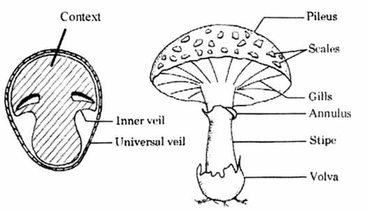
A universal veil is a temporary membranous tissue that fully envelops immature fruiting bodies of certain gilled mushrooms. The developing Caesar’s mushroom (Amanita caesarea), for example, which may resemble a small white sphere at this point, is protected by this structure. The veil will eventually rupture and disintegrate by the force of the expanding and maturing mushroom, but will usually leave evidence of its former shape with remnants. These remnants include the volva, or cup-like structure at the base of the stipe, and patches or “warts” on top of the cap (ref. [5])
A partial veil (also called an inner veil, to differentiate it from the “outer” veil, or velum[1]) is a temporary structure of tissue found on the fruiting bodies of some basidiomycete fungi, typically agarics. Its role is to isolate and protect the developing spore-producing surface, represented by gills or tubes, found on the lower surface of the cap. A partial veil, in contrast to a universal veil, extends from the stem surface to the cap edge. The partial veil later disintegrates, once the fruiting body has matured and the spores are ready for dispersal. It might then give rise to a stem ring, or fragments attached to the stem or cap edge. In some mushrooms, both a partial veil and a universal veil may be present (ref. [6]).
Mushroom Features by pictures
As shown by ref. [7], some pictures outline basic mushroom features as they can be found within our dataset.
Mushroom structure:
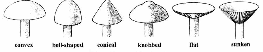
Mushroom cap shape:
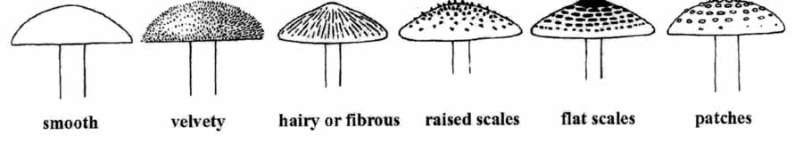
Mushroom cap surface:
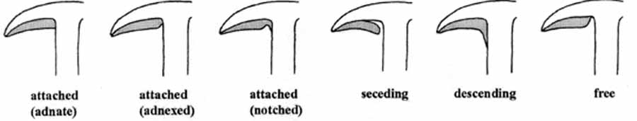
Mushroom gill attachment:
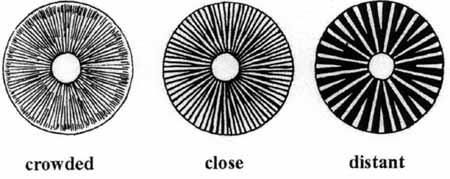
Mushroom gill spacing:
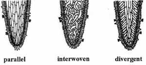
Mushroom gill tissue arrangement:
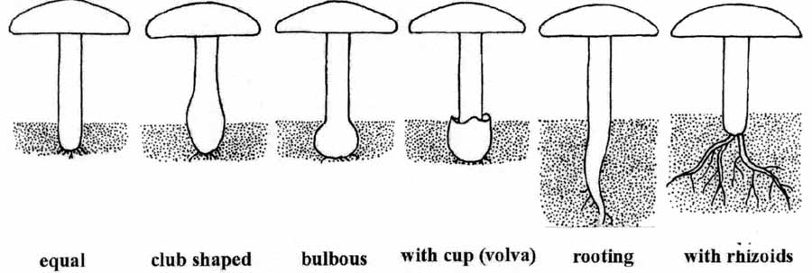
Mushroom stalk type:
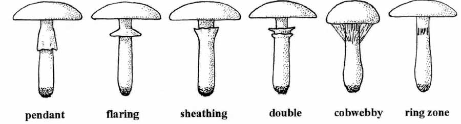
Mushroom ring type:
Exploratory Analysis
Packages
The overall list of packages used for this tutorial are as follows.
suppressPackageStartupMessages(library(caret))
suppressPackageStartupMessages(library(ggplot2))
suppressPackageStartupMessages(library(dplyr))
suppressPackageStartupMessages(library(gridExtra))
suppressPackageStartupMessages(library(Kmisc))
suppressPackageStartupMessages(library(gmodels))
suppressPackageStartupMessages(library(ggparallel))
suppressPackageStartupMessages(library(rpart.plot))
suppressPackageStartupMessages(library(sqldf))
Exploring Data
The dataset includes descriptions of hypothetical samples corresponding to 23 species of gilled mushrooms in the Agaricus and Lepiota Family. Each species is identified as definitely edible, definitely poisonous, or of unknown edibility and not recommended. This latter class was combined with the poisonous one (ref. [1]).
url_file <-  "https://archive.ics.uci.edu/ml/machine-learning-databases/mushroom/agaricus-lepiota.data"
mushrooms <- read.csv(url(url_file), header=FALSE)
dim(mushrooms)

[1] 8124   23
str(mushrooms)
'data.frame':	8124 obs. of  23 variables:
 $ V1 : Factor w/ 2 levels "e","p": 2 1 1 2 1 1 1 1 2 1 ...
 $ V2 : Factor w/ 6 levels "b","c","f","k",..: 6 6 1 6 6 6 1 1 6 1 ...
 $ V3 : Factor w/ 4 levels "f","g","s","y": 3 3 3 4 3 4 3 4 4 3 ...
 $ V4 : Factor w/ 10 levels "b","c","e","g",..: 5 10 9 9 4 10 9 9 9 10 ...
 $ V5 : Factor w/ 2 levels "f","t": 2 2 2 2 1 2 2 2 2 2 ...
....
....
According to dataset description, the first column represents the mushroom classification based on the two categories “edible” and “poisonous”. The other columns are:
- 1. cap-shape: bell=b, conical=c, convex=x, flat=f, knobbed=k, sunken=s
- 2. cap-surface: fibrous=f, grooves=g, scaly=y, smooth=s
- 3. cap-color: brown=n, buff=b, cinnamon=c, gray=g, green=r, pink=p, purple=u, red=e, white=w, yellow=y
- 4. bruises: bruises=t, no=f
- 5. odor: almond=a, anise=l, creosote=c, fishy=y, foul=f, musty=m, none=n, pungent=p, spicy=s
- 6. gill-attachment: attached=a, descending=d, free=f, notched=n
- 7. gill-spacing: close=c, crowded=w, distant=d
- 8. gill-size: broad=b, narrow=n
- 9. gill-color: black=k, brown=n, buff=b, chocolate=h, gray=g, green=r, orange=o, pink=p, purple=u, red=e, white=w, yellow=y
- 10. stalk-shape: enlarging=e, tapering=t
- 11. stalk-root: bulbous=b, club=c, cup=u, equal=e, rhizomorphs=z, rooted=r, missing=?
- 12. stalk-surface-above-ring: fibrous=f, scaly=y, silky=k, smooth=s
- 13. stalk-surface-below-ring: fibrous=f, scaly=y, silky=k, smooth=s
- 14. stalk-color-above-ring: brown=n, buff=b, cinnamon=c, gray=g, orange=o, pink=p, red=e, white=w, yellow=y
- 15. stalk-color-below-ring: brown=n, buff=b, cinnamon=c, gray=g, orange=o, pink=p, red=e, white=w, yellow=y
- 16. veil-type: partial=p, universal=u
- 17. veil-color: brown=n, orange=o, white=w, yellow=y
- 18. ring-number: none=n, one=o, two=t
- 19. ring-type: cobwebby=c, evanescent=e, flaring=f, large=l, none=n, pendant=p, sheathing=s, zone=z
- 20. spore-print-color: black=k, brown=n, buff=b, chocolate=h, green=r, orange=o, purple=u, white=w, yellow=y
- 21. population: abundant=a, clustered=c, numerous=n, scattered=s, several=v, solitary=y
- 22. habitat: grasses=g, leaves=l, meadows=m, paths=p, urban=u, waste=w, woods=d
fields <- c("class",
            "cap_shape",
            "cap_surface",
            "cap_color",
            "bruises",
            "odor",
            "gill_attachment",
            "gill_spacing",
            "gill_size",
            "gill_color",
            "stalk_shape",
            "stalk_root",
            "stalk_surface_above_ring",
            "stalk_surface_below_ring",
            "stalk_color_above_ring",
            "stalk_color_below_ring",
            "veil_type",
            "veil_color",
            "ring_number",
            "ring_type",
            "spore_print_color",
            "population",
            "habitat")
colnames(mushrooms) <- fields
head(mushrooms)
 class cap_shape cap_surface cap_color bruises odor gill_attachment gill_spacing gill_size gill_color
1     p         x           s         n       t    p               f            c         n          k
2     e         x           s         y       t    a               f            c         b          k
3     e         b           s         w       t    l               f            c         b          n
4     p         x           y         w       t    p               f            c         n          n
5     e         x           s         g       f    n               f            w         b          k
6     e         x           y         y       t    a               f            c         b          n
  stalk_shape stalk_root stalk_surface_above_ring stalk_surface_below_ring stalk_color_above_ring
1           e          e                        s                        s                      w
2           e          c                        s                        s                      w
3           e          c                        s                        s                      w
4           e          e                        s                        s                      w
5           t          e                        s                        s                      w
6           e          c                        s                        s                      w
  stalk_color_below_ring veil_type veil_color ring_number ring_type spore_print_color population habitat
1                      w         p          w           o         p                 k          s       u
2                      w         p          w           o         p                 n          n       g
3                      w         p          w           o         p                 n          n       m
4                      w         p          w           o         p                 k          s       u
5                      w         p          w           o         e                 n          a       g
6                      w         p          w           o         p                 k          n       g
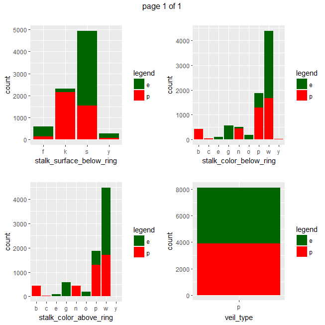
We observe that veil-type is equal to “partial” for all the mushrooms within our dataset. No NA’s values are present.
sum(complete.cases(mushrooms))
[1] 8124
mush_features <- colnames(mushrooms)[-1]
grid <- expand.grid(mush_features, mush_features, stringsAsFactors = FALSE)
grid = grid %>% filter(Var1 != Var2)
chunk <- nrow(grid)/length(mush_features)
gp <- invisible(lapply(mush_features, function(x) {
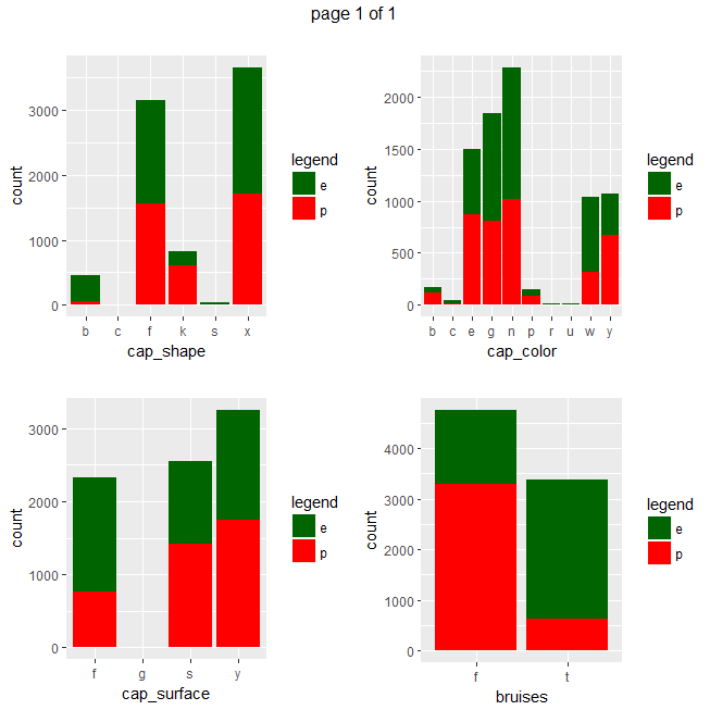
ggplot(data=mushrooms, aes(x = eval(parse(text=x)), fill = class)) + geom_bar() + xlab(x) + scale_fill_manual("legend", values = c("e" = "darkgreen", "p" = "red")) + ggtitle("")}))
grob_plots <- invisible(lapply(chunk(1, length(gp), 4), function(x) {
marrangeGrob(grobs=lapply(gp[x], ggplotGrob), nrow=2, ncol=2)}))
grob_plots
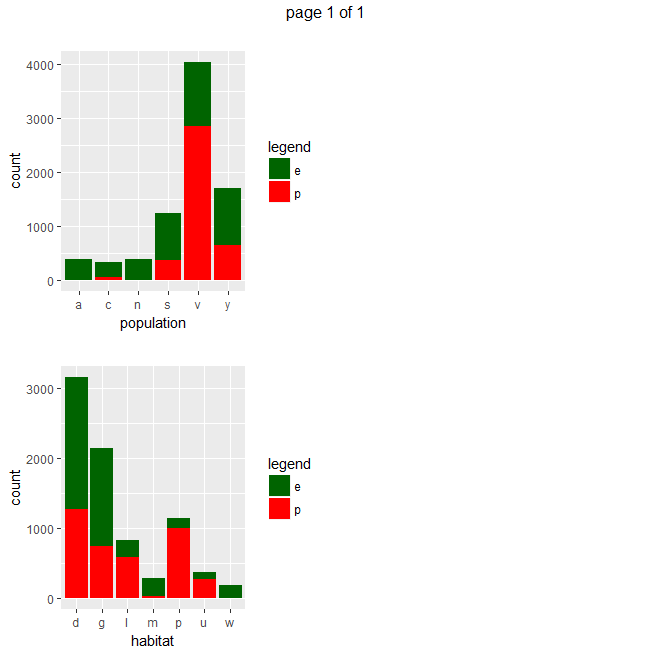
Gives a series of 2×2 barplots as shown below:
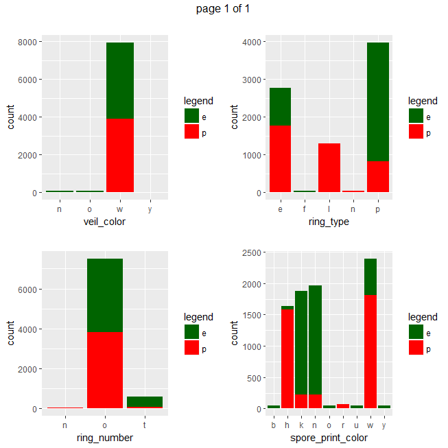
Contingence tables are useful for revealing how edible/poisonous mushrooms are segmented across their dataset features.
table_res <- lapply(mush_features, function(x) {table(mushrooms$class, mushrooms[,x])})
names(table_res) <- mush_features
table_res

$cap_shape
       b    c    f    k    s    x
  e  404    0 1596  228   32 1948
  p   48    4 1556  600    0 1708

$cap_surface
       f    g    s    y
  e 1560    0 1144 1504
  p  760    4 1412 1740

$cap_color
       b    c    e    g    n    p    r    u    w    y
  e   48   32  624 1032 1264   56   16   16  720  400
  p  120   12  876  808 1020   88    0    0  320  672
...
...
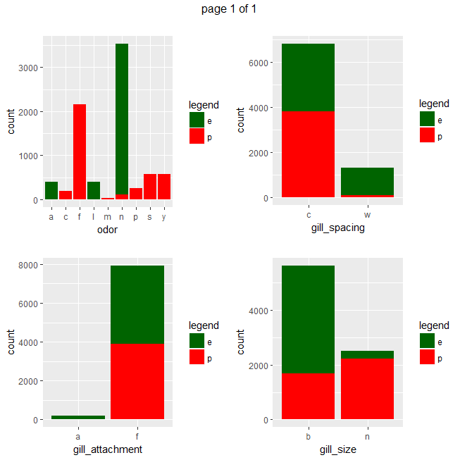
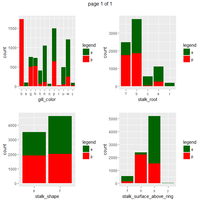
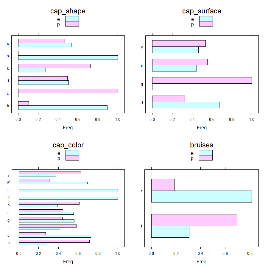
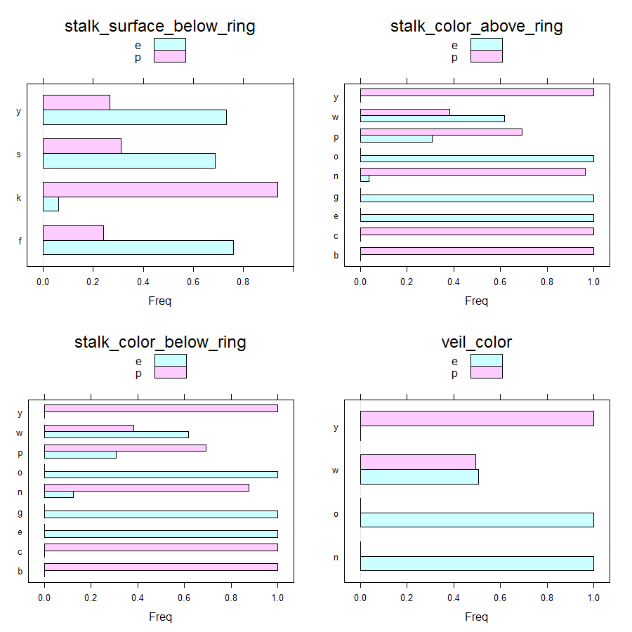
Main insights resulting from above barplots and contingency tables are:
- * only poisonous mushrooms have convex cap-shape; only edible mushrooms have sunken cap-shape
- * only poisonous mushrooms have cap-surface with grooves
- * only edible mushrooms have green or purple cap-color
- * odor is strongly indicative of what mushrooms are (edible/poisonous)
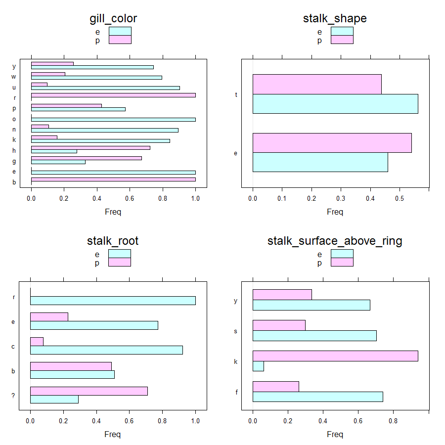
- * only poisonous mushrooms have buff or green gill color
- * only edible mushrooms have red or orange gill color
- * only edible mushrooms have rooted stalk root
- * stalk_color_above_ring and stalk_color_below_ring are relevant features for out classification problem
- * only edible mushrooms have brown veil color
- * only poisonous mushrooms have yellow veil color
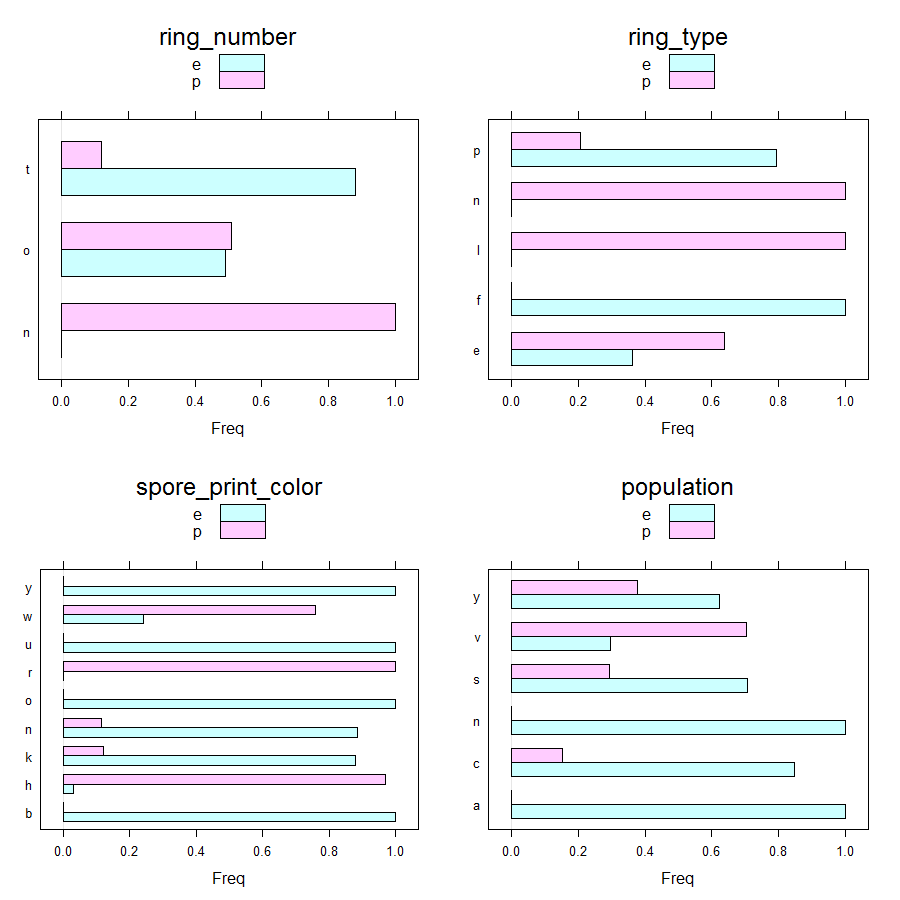
- * only poisonous mushrooms do not have rings
- * only edible mushrooms have flaring ring type
- * only poisonous mushrooms have none ring type
- * only edible mushrooms have black, orange, purple or yellow spore print color
- * only poisonous mushrooms have green spore print color
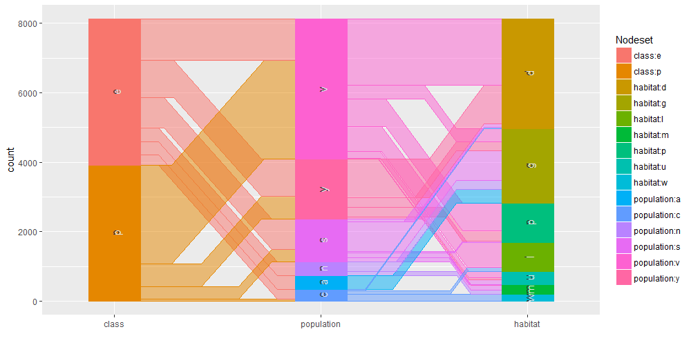
- * only edible mushrooms have abundant or numerous population
- * only edible musrooms have waste type habitat
Now we run a chi-square test in order to check for the significative relationship between mushroom features and their classification as edible or poisonous.
chisq_test_res = list()
relevant_features = c()

for (i in 2:length(colnames(mushrooms))) {
  if (nlevels(mushrooms[,i]) > 1) {
    fname = colnames(mushrooms)[i]
    res = chisq.test(mushrooms[,i], mushrooms[,"class"], simulate.p.value = TRUE)
    res$data.name = paste(fname, "class", sep= " and ")
    chisq_test_res[[fname]] = res
    relevant_features = c(relevant_features, fname)
  }
}
The check on factor levels is necessary as veil_type has got just one. Results are shown below.
chisq_test_res
$cap_shape

	Pearson's Chi-squared test with simulated p-value (based on 2000
	replicates)

data:  cap_shape and class
X-squared = 489.92, df = NA, p-value = 0.0004998


$cap_surface

	Pearson's Chi-squared test with simulated p-value (based on 2000
	replicates)
...
...
Based on reported p-values, all features having at least two levels are significative.
The veil_type is the only categorical feature with one level, as confirmed below.
setdiff(mush_features, relevant_features)
[1] "veil_type"
Barcharts can be obtained as follows.
barchart_plot <- lapply(relevant_features, function(x) {
  wgd <- CrossTable(mushrooms[,x], mushrooms$class, prop.chisq=F)
  barchart(wgd$prop.row, stack=F, auto.key=list(rectangles = TRUE, space = "top", title = x))
})
names(barchart_plot) <- relevant_features

par(mfrow=c(2,2))
seq_i <- seq(1, length(barchart_plot)-4, by=4)
for (i in seq_i) {
  grid.arrange(barchart_plot[[i]],
               barchart_plot[[i+1]],
               barchart_plot[[i+2]],
               barchart_plot[[i+3]],
               nrow=2,
               ncol=2)
}
Gives the following plots.
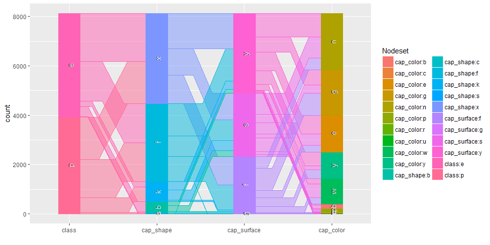
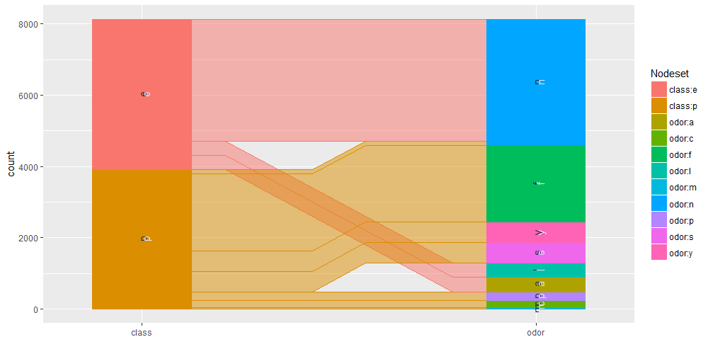
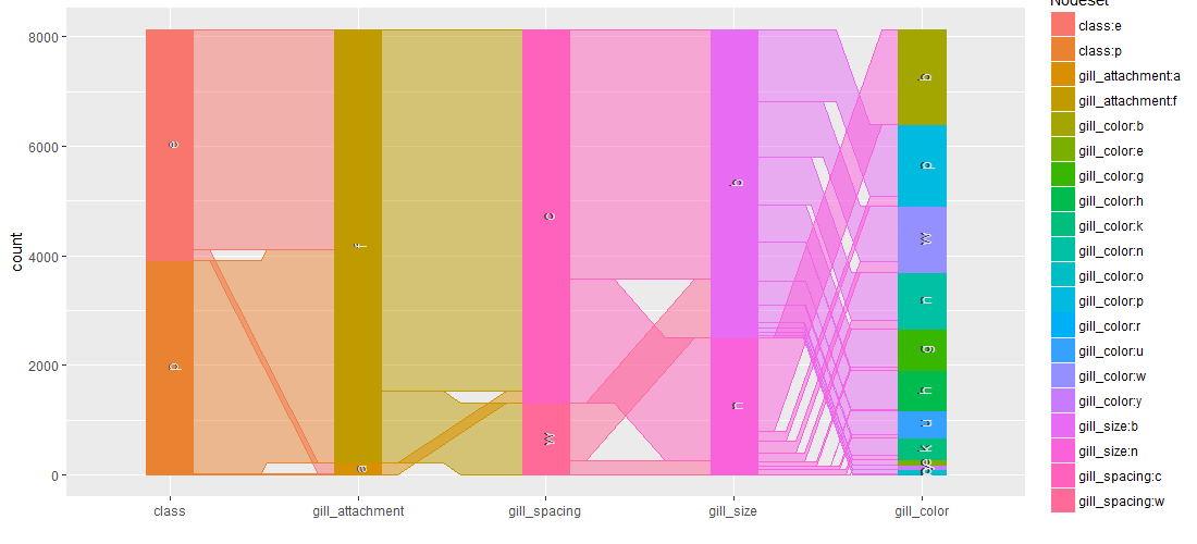
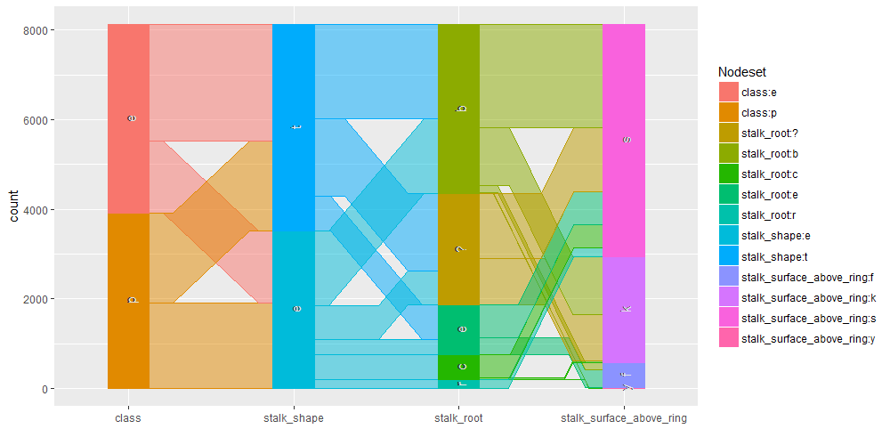
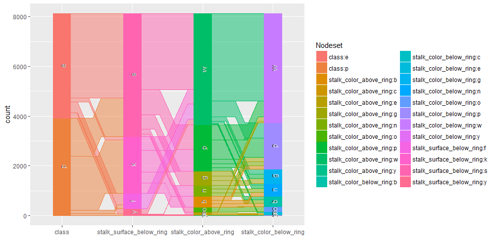
Common angle plots as provided within ggparallel package may help in visualizing categorical data.
ggparallel(list("class", relevant_features[1:3]), data=mushrooms)
Gives this plot.
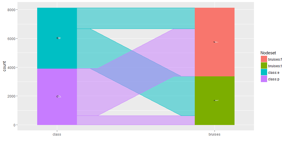
ggparallel(list("class", relevant_features[4]), data=mushrooms)
Gives this plot.
ggparallel(list("class", relevant_features[5]), data=mushrooms)
Gives this plot.
ggparallel(list("class", relevant_features[6:9]), data=mushrooms)
Gives this plot.
ggparallel(list("class", relevant_features[10:12]), data=mushrooms)
Gives this plot.
ggparallel(list("class", relevant_features[13:15]), data=mushrooms)
Gives this plot.
ggparallel(list("class", relevant_features[16]), data=mushrooms)
Gives this plot.
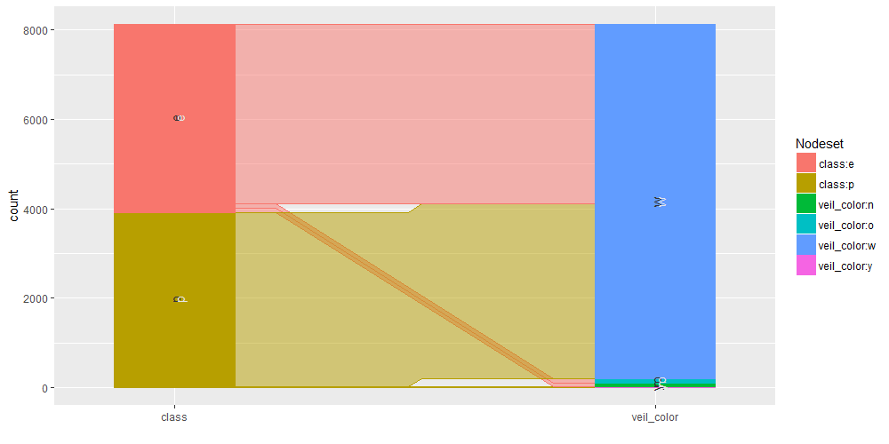
ggparallel(list("class", relevant_features[17:18]), data=mushrooms)
Gives this plot.
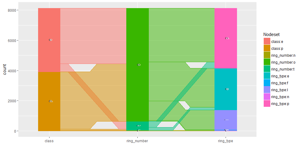
ggparallel(list("class", relevant_features[19]), data=mushrooms)
Gives this plot.
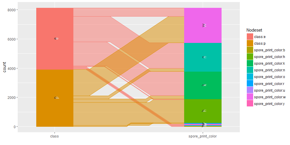
ggparallel(list("class", relevant_features[20:21]), data=mushrooms)
Gives this plot.
It is as well interesting to perform query on the mushroom database to analyse specific subset of the overall available information. We are going to show some example using facilities within the sqldf R package.
For example, herein we create a new dataset having class and cap_shape columns to report mushrooms with no odor.
query_1 <- sqldf("select class,cap_shape from mushrooms where odor =='n'")
class(query_1)
[1] "data.frame"
head(query_1)
  class cap_shape
1     e         x
2     e         x
3     e         s
4     e         f
5     e         f
6     e         s
table(query_1)
   cap_shape
class    b    c    f    k    s    x
    e  148    0 1452  228   32 1548
    p   48    4   48   12    0    8
Further example queries are shown.
query_2 <- sqldf("select class,cap_color from mushrooms where stalk_shape =='e' and stalk_root = 'b'")
table(query_2)
 cap_color
class   b   c   e   g   n   p   r   u   w   y
    e   0  32   0   8  48   8   0   0   0   0
    p  24   0   0 712   0  88   0   0  96 648
query_3 <- sqldf("select class,cap_shape from mushrooms where odor == 'n' and ring_number = 'o'")
table(query_3)
 cap_shape
class    b    c    f    k    s    x
    e   48    0 1368   64   32 1368
    p   12    4   12   12    0    8
query_3 <- sqldf("select class,cap_shape from mushrooms where odor == 'n' and ring_number = 'o'")
table(query_3)
 cap_shape
class    b    c    f    k    s    x
    e   48    0 1368   64   32 1368
    p   12    4   12   12    0    8
Datasets obtained by sqldf select operations can also be reused as input of further queries.
query_4 <- sqldf("select class,cap_shape,ring_number from mushrooms where odor =='n'")
query_4_1 <- sqldf("select class,cap_shape from query_4 where ring_number =='o'")

identical(query_3, query_4_1)
[1] TRUE
Conclusions
Datastory telling offers the chance to gain domain knowledge on new fields. We ran exploratory analysis by taking advantage of more than one visualization tool, contingency tables and SQL queries. If you have any questions, please feel free to comment below.
You can find the part 2 of this post here.
References
-
[1] UCI Machine Learning Archive – Mushroom Dataset
[2] Wikipedia – Mushroom Tutorial
[3] Mushroom Anatomy
[4] Identify Mushrooms
[5] Wikipedia – Universal Veil
[6] Wikipedia – Partial Veil
[7] Mushroom Glossary
[8] Caret package site
[9] rpart package vignette
[10] C5.0 package vignette
[11] C5.0: An Informal Tutorial
[12] Caret Package Vignette
[13] How Decision Tree Algorithms Works