In the present tutorial, I show an introductory text analysis of a ABC-news news headlines dataset. I will have a look to the most common words therein present and run a sentiment analysis on those headlines by taking advantage of the following sentiment lexicons:
- NRC
- Bing
- AFINN
The NRC sentiment lexicon from Saif Mohammad and Peter Turney categorizes words into categories of positive, negative, anger, anticipation, disgust, fear joy, sadness, surprise and trust.
The Bing sentiment lexicon from Bing Liu and others categorizes words into positive or negative sentiment category.
The AFINN sentiment lexicon from Finn Arup Nielsen assigns words with a score from -5 to 5, with negative scores indicating negative sentiment and positive scores indicating positive sentiment.
For more information about those sentiment lexicons, see references listed out at the bottom.
Packages
I am going to take advantage of the following R packages.
suppressPackageStartupMessages(library(stringr))
suppressPackageStartupMessages(library(dplyr))
suppressPackageStartupMessages(library(tidytext))
suppressPackageStartupMessages(library(tidyr))
suppressPackageStartupMessages(library(textdata))
suppressPackageStartupMessages(library(widyr))
suppressPackageStartupMessages(library(ggplot2))
Packages versions are herein listed.
packages <- c("stringr", "dplyr", "tidytext", "tidyr", "textdata", "widyr", "ggplot2")
version <- lapply(packages, packageVersion)
version_c <- do.call(c, version)
data.frame(packages=packages, version = as.character(version_c))
##   packages version
## 1  stringr   1.4.0
## 2    dplyr   0.8.4
## 3 tidytext   0.2.2
## 4    tidyr   1.0.2
## 5 textdata   0.3.0
## 6    widyr   0.1.2
## 7  ggplot2   3.2.1
Running on Windows-10 the following R language version.
R.version
##                _
## platform       x86_64-w64-mingw32
## arch           x86_64
## os             mingw32
## system         x86_64, mingw32
## status
## major          3
## minor          5.3
## year           2019
## month          03
## day            11
## svn rev        76217
## language       R
## version.string R version 3.5.3 (2019-03-11)
## nickname       Great Truth
Note
Before running this code, make sure to have downloaded the lexicon of the sentiments baselines in use by executing the following operations:
get_sentiments("nrc")
get_sentiments("bing")
get_sentiments("afinn")
and accepting all prescriptions as asked by the interactive menu showing up.
Getting Data
I then download our news dataset containing millions of headlines from:
“https://www.kaggle.com/therohk/million-headlines/downloads/million-headlines.zip/7”
Its uncompression produces the abcnews-date-text.csv file. I load it into the news_data dataset and have a look at.
news_data <- read.csv("abcnews-date-text.csv", header = TRUE, stringsAsFactors = FALSE)
dim(news_data)
## [1] 1103663       2
head(news_data)
##   publish_date                                      headline_text
## 1     20030219 aba decides against community broadcasting licence
## 2     20030219     act fire witnesses must be aware of defamation
## 3     20030219     a g calls for infrastructure protection summit
## 4     20030219           air nz staff in aust strike for pay rise
## 5     20030219      air nz strike to affect australian travellers
## 6     20030219                  ambitious olsson wins triple jump
tail(news_data)
##         publish_date                                               headline_text
## 1103658     20171231             stunning images from the sydney to hobart yacht
## 1103659     20171231 the ashes smiths warners near miss liven up boxing day test
## 1103660     20171231                     timelapse: brisbanes new year fireworks
## 1103661     20171231                    what 2017 meant to the kids of australia
## 1103662     20171231            what the papodopoulos meeting may mean for ausus
## 1103663     20171231   who is george papadopoulos the former trump campaign aide
Token Analysis
It is time to extract the tokens from our dataset. Select the column named as headline_text and unnesting the word tokens determine the following.
news_df <- news_data %>% select(headline_text)
news_tokens <- news_df %>% unnest_tokens(word, headline_text)
head(news_tokens, 10)
##             word
## 1            aba
## 1.1      decides
## 1.2      against
## 1.3    community
## 1.4 broadcasting
## 1.5      licence
## 2            act
## 2.1         fire
## 2.2    witnesses
## 2.3         must
tail(news_tokens, 10)
##                   word
## 1103662.7        ausus
## 1103663            who
## 1103663.1           is
## 1103663.2       george
## 1103663.3 papadopoulos
## 1103663.4          the
## 1103663.5       former
## 1103663.6        trump
## 1103663.7     campaign
## 1103663.8         aide
It is interesting to generate and inspect a table reporting how many times each token shows up within the headlines and its proportion with respect the total.
news_tokens_count <- news_tokens %>% count(word, sort = TRUE) %>% mutate(proportion = n / sum(n))
The top-10 words which appear most.
head(news_tokens_count, 10)
## # A tibble: 10 x 3
##    word        n proportion
##    <chr>   <int>      <dbl>
##  1 to     214201    0.0303
##  2 in     135981    0.0192
##  3 for    130239    0.0184
##  4 of      80759    0.0114
##  5 on      73037    0.0103
##  6 over    50306    0.00711
##  7 the     49810    0.00704
##  8 police  35984    0.00509
##  9 at      31723    0.00449
## 10 with    29676    0.00420
And the ones which appear less frequently:
tail(news_tokens_count, 10)
## # A tibble: 10 x 3
##    word           n  proportion
##    <chr>      <int>       <dbl>
##  1 zweli          1 0.000000141
##  2 zwitkowsky     1 0.000000141
##  3 zydelig        1 0.000000141
##  4 zygar          1 0.000000141
##  5 zygiefs        1 0.000000141
##  6 zylvester      1 0.000000141
##  7 zynga          1 0.000000141
##  8 zyngier        1 0.000000141
##  9 zz             1 0.000000141
## 10 zzz            1 0.000000141
There is an issue in having doing that way. The issue is that there are words which do not have relevant role in easing the sentiment analysis, the so called stop words. Herein below the stop words wihin our dataset are shown.
data(stop_words)
head(stop_words, 10)
## # A tibble: 10 x 2
##    word        lexicon
##    <chr>       <chr>
##  1 a           SMART
##  2 a's         SMART
##  3 able        SMART
##  4 about       SMART
##  5 above       SMART
##  6 according   SMART
##  7 accordingly SMART
##  8 across      SMART
##  9 actually    SMART
## 10 after       SMART
To remove stop words as required, we take advantage of the anti_join operation.
news_tokens_no_sp <- news_tokens %>% anti_join(stop_words)
head(news_tokens_no_sp, 10)
##            word
## 1           aba
## 2       decides
## 3     community
## 4  broadcasting
## 5       licence
## 6           act
## 7          fire
## 8     witnesses
## 9         aware
## 10   defamation
Then, counting news tokens again after having removed the stop words.
news_tokens_count <- news_tokens_no_sp %>% count(word, sort = TRUE) %>% mutate(proportion = n / sum(n))
head(news_tokens_count, 10)
## # A tibble: 10 x 3
##    word          n proportion
##    <chr>     <int>      <dbl>
##  1 police    35984    0.00673
##  2 govt      16923    0.00317
##  3 court     16380    0.00306
##  4 council   16343    0.00306
##  5 interview 15025    0.00281
##  6 fire      13910    0.00260
##  7 nsw       12912    0.00242
##  8 australia 12353    0.00231
##  9 plan      12307    0.00230
## 10 water     11874    0.00222
tail(news_tokens_count)
## # A tibble: 6 x 3
##   word          n  proportion
##   <chr>     <int>       <dbl>
## 1 zygiefs       1 0.000000187
## 2 zylvester     1 0.000000187
## 3 zynga         1 0.000000187
## 4 zyngier       1 0.000000187
## 5 zz            1 0.000000187
## 6 zzz           1 0.000000187
Then, I filter out tokens having more than 8,000 counts.
news_token_over8000 <- news_tokens_count %>% filter(n > 8000) %>% mutate(word = reorder(word, n))
nrow(news_token_over8000)
## [1] 32
head(news_token_over8000, 10)
## # A tibble: 10 x 3
##    word          n proportion
##    <fct>     <int>      <dbl>
##  1 police    35984    0.00673
##  2 govt      16923    0.00317
##  3 court     16380    0.00306
##  4 council   16343    0.00306
##  5 interview 15025    0.00281
##  6 fire      13910    0.00260
##  7 nsw       12912    0.00242
##  8 australia 12353    0.00231
##  9 plan      12307    0.00230
## 10 water     11874    0.00222
tail(news_token_over8000, 10)
## # A tibble: 10 x 3
##    word         n proportion
##    <fct>    <int>      <dbl>
##  1 day       8818    0.00165
##  2 hospital  8815    0.00165
##  3 car       8690    0.00163
##  4 coast     8411    0.00157
##  5 calls     8401    0.00157
##  6 win       8315    0.00156
##  7 woman     8213    0.00154
##  8 killed    8129    0.00152
##  9 accused   8094    0.00151
## 10 world     8087    0.00151
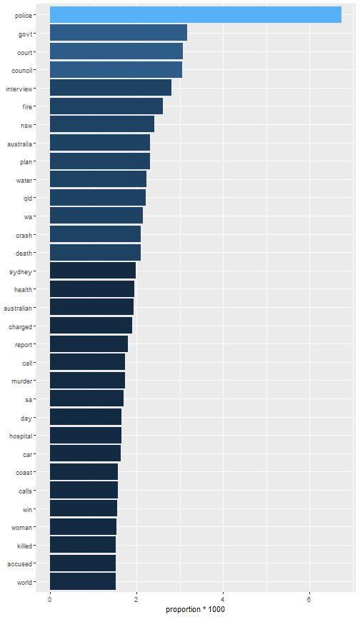
It is interesting to show the proportion as per-thousands by means of an histogram plot.
news_token_over8000 %>%
  ggplot(aes(word, proportion*1000, fill=ceiling(proportion*1000))) +
  geom_col() + xlab(NULL) + coord_flip() + theme(legend.position = "none")
News Sentiment Analysis
In this paragraph, I focus on each single headline to evaluate its specific sentiment as determined by each lexicon. Hence the output shall determine if each specific headline has got positive or negative sentiment.
head(news_df, 10)
##                                         headline_text
## 1  aba decides against community broadcasting licence
## 2      act fire witnesses must be aware of defamation
## 3      a g calls for infrastructure protection summit
## 4            air nz staff in aust strike for pay rise
## 5       air nz strike to affect australian travellers
## 6                   ambitious olsson wins triple jump
## 7          antic delighted with record breaking barca
## 8   aussie qualifier stosur wastes four memphis match
## 9        aust addresses un security council over iraq
## 10         australia is locked into war timetable opp
I will analyse only the first 1000 headlines just for computational time reasons. The token list of such is as follows.
news_df_subset <- news_df[1:1000,,drop=FALSE]
tkn_l <- apply(news_df_subset, 1, function(x) { data.frame(headline_text=x, stringsAsFactors = FALSE) %>% unnest_tokens(word, headline_text)})
Removing the stop words from the token list.
single_news_tokens <- lapply(tkn_l, function(x) {anti_join(x, stop_words)})
str(single_news_tokens, list.len = 5)
## List of 1000
##  $ 1   :'data.frame':    5 obs. of  1 variable:
##   ..$ word: chr [1:5] "aba" "decides" "community" "broadcasting" ...
##  $ 2   :'data.frame':    5 obs. of  1 variable:
##   ..$ word: chr [1:5] "act" "fire" "witnesses" "aware" ...
##  $ 3   :'data.frame':    4 obs. of  1 variable:
##   ..$ word: chr [1:4] "calls" "infrastructure" "protection" "summit"
##  $ 4   :'data.frame':    7 obs. of  1 variable:
##   ..$ word: chr [1:7] "air" "nz" "staff" "aust" ...
##  $ 5   :'data.frame':    6 obs. of  1 variable:
##   ..$ word: chr [1:6] "air" "nz" "strike" "affect" ...
##   [list output truncated]
As we can see, to each headline is associated a list of tokens. The sentiment of a headline is computed as based on the sum of positive/negative score of each token of.
single_news_tokens[[1]]
##           word
## 1          aba
## 2      decides
## 3    community
## 4 broadcasting
## 5      licence
Bing lexicon
In this paragraph, the computation of the sentiment associated to the tokens list is shown for Bing lexicon. I first define a function named as compute_sentiment() whose purpose is to output the positiveness score of a specific headline.
compute_sentiment <- function(d) {
  if (nrow(d) == 0) {
    return(NA)
  }
  neg_score <- d %>% filter(sentiment=="negative") %>% nrow()
  pos_score <- d %>% filter(sentiment=="positive") %>% nrow()
  pos_score - neg_score
}
The inner join on bing lexicon of each single headline tokens list is given as input to the compute_sentiment() function to determine the sentiment score of each specific headline.
sentiments_bing <- get_sentiments("bing")
str(sentiments_bing)
## Classes 'tbl_df', 'tbl' and 'data.frame':    6786 obs. of  2 variables:
##  $ word     : chr  "2-faces" "abnormal" "abolish" "abominable" ...
##  $ sentiment: chr  "negative" "negative" "negative" "negative" ...
single_news_sentiment_bing <- sapply(single_news_tokens, function(x) { x %>% inner_join(sentiments_bing) %>% compute_sentiment()})
The result is a vector of integers each element value at i-th position is the sentiment associated to the i-th news
str(single_news_sentiment_bing)
##  Named int [1:1000] NA -1 1 -1 -1 2 0 NA NA NA ...
##  - attr(*, "names")= chr [1:1000] "1" "2" "3" "4" ...
Here is the summary, please note that:
- the median is negative
- NA's show up
summary(single_news_sentiment_bing)
##    Min. 1st Qu.  Median    Mean 3rd Qu.    Max.    NA's
##  -3.000  -1.000  -1.000  -0.475   1.000   2.000     520
Collecting the resulting in a data frame as follows.
single_news_sentiment_bing_df <- data.frame(headline_text=news_df_subset$headline_text, score = single_news_sentiment_bing)
head(single_news_sentiment_bing_df, 10)
##                                         headline_text score
## 1  aba decides against community broadcasting licence    NA
## 2      act fire witnesses must be aware of defamation    -1
## 3      a g calls for infrastructure protection summit     1
## 4            air nz staff in aust strike for pay rise    -1
## 5       air nz strike to affect australian travellers    -1
## 6                   ambitious olsson wins triple jump     2
## 7          antic delighted with record breaking barca     0
## 8   aussie qualifier stosur wastes four memphis match    NA
## 9        aust addresses un security council over iraq    NA
## 10         australia is locked into war timetable opp    NA
NRC lexicon
In this paragraph, the computation of the sentiment associated to the tokens list is shown for NRC lexicon. With respect the previous analysis based on bing lexicon, some more pre-processing is needed as explained in what follows. First we get the NRC sentiment lexicon and see what are the sentiments threin present.
sentiments_nrc <- get_sentiments("nrc")
(unique_sentiments_nrc <- unique(sentiments_nrc$sentiment))
##  [1] "trust"        "fear"         "negative"     "sadness"      "anger"        "surprise"
##  [7] "positive"     "disgust"      "joy"          "anticipation"
To have as output a positive/negative sentiment result, I define a mapping of abovelisted sentiments to a positive/negative string result as follows.
compute_pos_neg_sentiments_nrc <- function(the_sentiments_nrc) {
  s <- unique(the_sentiments_nrc$sentiment)
  df_sentiments <- data.frame(sentiment = s,
                              mapped_sentiment = c("positive", "negative", "negative", "negative",
                                                    "negative", "positive", "positive", "negative",
                                                    "positive", "positive"))
  ss <- sentiments_nrc %>% inner_join(df_sentiments)
  the_sentiments_nrc$sentiment <- ss$mapped_sentiment
  the_sentiments_nrc
}

nrc_sentiments_pos_neg_scale <- compute_pos_neg_sentiments_nrc(sentiments_nrc)
Above function is used to produce the single headline text sentiment results. Such result is given as input to the compute_sentiment() function.
single_news_sentiment_nrc <- sapply(single_news_tokens, function(x) { x %>% inner_join(nrc_sentiments_pos_neg_scale) %>% compute_sentiment()})
str(single_news_sentiment_nrc)
##  Named int [1:1000] 1 -4 1 2 -2 2 4 NA 5 -2 ...
##  - attr(*, "names")= chr [1:1000] "1" "2" "3" "4" ...
Here is the summary, please note that:
- the median is equal to zero
- NA's show up
summary(single_news_sentiment_nrc)
##    Min. 1st Qu.  Median    Mean 3rd Qu.    Max.    NA's
## -9.0000 -2.0000  0.0000 -0.3742  2.0000  9.0000     257
single_news_sentiment_nrc_df <- data.frame(headline_text=news_df_subset$headline_text, score = single_news_sentiment_nrc)
head(single_news_sentiment_nrc_df, 10)
##                                         headline_text score
## 1  aba decides against community broadcasting licence     1
## 2      act fire witnesses must be aware of defamation    -4
## 3      a g calls for infrastructure protection summit     1
## 4            air nz staff in aust strike for pay rise     2
## 5       air nz strike to affect australian travellers    -2
## 6                   ambitious olsson wins triple jump     2
## 7          antic delighted with record breaking barca     4
## 8   aussie qualifier stosur wastes four memphis match    NA
## 9        aust addresses un security council over iraq     5
## 10         australia is locked into war timetable opp    -2
AFINN lexicon
In this paragraph, the computation of the sentiment associated to the tokens list is shown for AFINN lexicon.
sentiments_afinn <- get_sentiments("afinn")
colnames(sentiments_afinn) <- c("word", "sentiment")
str(sentiments_afinn)
## Classes 'spec_tbl_df', 'tbl_df', 'tbl' and 'data.frame': 2477 obs. of  2 variables:
##  $ word     : chr  "abandon" "abandoned" "abandons" "abducted" ...
##  $ sentiment: num  -2 -2 -2 -2 -2 -2 -3 -3 -3 -3 ...
##  - attr(*, "spec")=
##   .. cols(
##   ..   word = col_character(),
##   ..   value = col_double()
##   .. )
As we can see, the afinn lexicon provides a score for each token. We just need to sum up each headline tokens score to obtain the sentiment score of the headline under analysis.
single_news_sentiment_afinn_df <- lapply(single_news_tokens, function(x) { x %>% inner_join(sentiments_afinn)})
single_news_sentiment_afinn <- sapply(single_news_sentiment_afinn_df, function(x) {
      ifelse(nrow(x) > 0, sum(x$sentiment), NA)
  })
str(single_news_sentiment_afinn)
##  Named num [1:1000] NA -2 NA -2 -1 6 3 NA NA -2 ...
##  - attr(*, "names")= chr [1:1000] "1" "2" "3" "4" ...
Here is the summary, please note that:
- the median is negative
- NA's show up
summary(single_news_sentiment_afinn)
##    Min. 1st Qu.  Median    Mean 3rd Qu.    Max.    NA's
##  -9.000  -3.000  -2.000  -1.148   1.000   7.000     508
single_news_sentiment_afinn_df <- data.frame(headline_text=news_df_subset$headline_text, score = single_news_sentiment_afinn)
head(single_news_sentiment_afinn_df, 10)
##                                         headline_text score
## 1  aba decides against community broadcasting licence    NA
## 2      act fire witnesses must be aware of defamation    -2
## 3      a g calls for infrastructure protection summit    NA
## 4            air nz staff in aust strike for pay rise    -2
## 5       air nz strike to affect australian travellers    -1
## 6                   ambitious olsson wins triple jump     6
## 7          antic delighted with record breaking barca     3
## 8   aussie qualifier stosur wastes four memphis match    NA
## 9        aust addresses un security council over iraq    NA
## 10         australia is locked into war timetable opp    -2
Comparing results
Having obtained for each news three potential results as sentiment evaluation, we would like to compare their congruency.
As congruence we mean the fact that all three lexicons express the same positive or negative result, in other words the same score sign indipendently from its magnitude. If NA values are present, the congruence shall be computed until at least two non NA values are available, otherwise is equal to NA.
Furthermore we compute the final news sentiment as based upon the sum of each lexicon sentiment score.
compute_congruence <- function(x,y,z) {
  v <- c(sign(x), sign(y), sign(z))
  # if only one lexicon reports the score, we cannot check for congruence
  if (sum(is.na(v)) >= 2) {
    return (NA)
  }
  # removing NA and zero value
  v <- na.omit(v)
  v_sum <- sum(v)
  abs(v_sum) == length(v)
}

compute_final_sentiment <- function(x,y,z) {
  if (is.na(x) && is.na(y) && is.na(z)) {
    return (NA)
  }

  s <- sum(x, y, z, na.rm=TRUE)
  # positive sentiments have score strictly greater than zero
  # negative sentiments have score strictly less than zero
  # neutral sentiments have score equal to zero
  ifelse(s > 0, "positive", ifelse(s < 0, "negative", "neutral"))
}

news_sentiments_results <- data.frame(headline_text = news_df_subset$headline_text,
                                      bing_score = single_news_sentiment_bing,
                                      nrc_score = single_news_sentiment_nrc,
                                      afinn_score = single_news_sentiment_afinn,
                                      stringsAsFactors = FALSE)

news_sentiments_results <- news_sentiments_results %>% rowwise() %>%
  mutate(final_sentiment = compute_final_sentiment(bing_score, nrc_score, afinn_score),
         congruence = compute_congruence(bing_score, nrc_score, afinn_score))

head(news_sentiments_results, 40)
## Source: local data frame [40 x 6]
## Groups: <by row>
##
## # A tibble: 40 x 6
##    headline_text                           bing_score nrc_score afinn_score final_sentiment congruence
##    <chr>                                        <int>     <int>       <dbl> <chr>           <lgl>
##  1 aba decides against community broadcas~         NA         1          NA positive        NA
##  2 act fire witnesses must be aware of de~         -1        -4          -2 negative        TRUE
##  3 a g calls for infrastructure protectio~          1         1          NA positive        TRUE
##  4 air nz staff in aust strike for pay ri~         -1         2          -2 negative        FALSE
##  5 air nz strike to affect australian tra~         -1        -2          -1 negative        TRUE
##  6 ambitious olsson wins triple jump                2         2           6 positive        TRUE
##  7 antic delighted with record breaking b~          0         4           3 positive        FALSE
##  8 aussie qualifier stosur wastes four me~         NA        NA          NA <NA>            NA
##  9 aust addresses un security council ove~         NA         5          NA positive        NA
## 10 australia is locked into war timetable~         NA        -2          -2 negative        TRUE
## # ... with 30 more rows
Is would be useful to replace the numeric score with same {negative, neutral, positive} scale.
replace_score_with_sentiment <- function(v_score) {
  v_score[v_score > 0] <- "positive"
  v_score[v_score < 0] <- "negative"
  v_score[v_score == 0] <- "neutral"
  v_score
}

news_sentiments_results$bing_score <- replace_score_with_sentiment(news_sentiments_results$bing_score)
news_sentiments_results$nrc_score <- replace_score_with_sentiment(news_sentiments_results$nrc_score)
news_sentiments_results$afinn_score <- replace_score_with_sentiment(news_sentiments_results$afinn_score)

news_sentiments_results[,2:5] <- lapply(news_sentiments_results[,2:5], as.factor)

head(news_sentiments_results, 40)
## Source: local data frame [40 x 6]
## Groups: <by row>
##
## # A tibble: 40 x 6
##    headline_text                           bing_score nrc_score afinn_score final_sentiment congruence
##    <chr>                                   <fct>      <fct>     <fct>       <fct>           <lgl>
##  1 aba decides against community broadcas~ <NA>       positive  <NA>        positive        NA
##  2 act fire witnesses must be aware of de~ negative   negative  negative    negative        TRUE
##  3 a g calls for infrastructure protectio~ positive   positive  <NA>        positive        TRUE
##  4 air nz staff in aust strike for pay ri~ negative   positive  negative    negative        FALSE
##  5 air nz strike to affect australian tra~ negative   negative  negative    negative        TRUE
##  6 ambitious olsson wins triple jump       positive   positive  positive    positive        TRUE
##  7 antic delighted with record breaking b~ neutral    positive  positive    positive        FALSE
##  8 aussie qualifier stosur wastes four me~ <NA>       <NA>      <NA>        <NA>            NA
##  9 aust addresses un security council ove~ <NA>       positive  <NA>        positive        NA
## 10 australia is locked into war timetable~ <NA>       negative  negative    negative        TRUE
## # ... with 30 more rows
Tabularizations of each lexicon resulting sentiment and final sentiments are herein shown.
table(news_sentiments_results$bing_score, news_sentiments_results$final_sentiment, dnn = c("bing", "final"))
##           final
## bing       negative neutral positive
##   negative      278      15       14
##   neutral        16       6       11
##   positive        6       7      127
table(news_sentiments_results$nrc_score, news_sentiments_results$final_sentiment, dnn = c("nrc", "final"))
##           final
## nrc        negative neutral positive
##   negative      353      10        4
##   neutral        18      13        6
##   positive       25      16      298
table(news_sentiments_results$afinn_score, news_sentiments_results$final_sentiment, dnn = c("afinn", "final"))
##           final
## afinn      negative neutral positive
##   negative      326      10       12
##   neutral         3       1        6
##   positive        4       9      121
Tabularization of congruence and final sentiments is herein shown.
table(news_sentiments_results$congruence, news_sentiments_results$final_sentiment, dnn = c("congruence", "final"))
##           final
## congruence negative neutral positive
##      FALSE       67      33       45
##      TRUE       292       0      132
Conclusions
We analyzed the news headlines to determine their sentiments while taking advantage of three sentiments lexicons. We outlined some basics of the methodology for such purpose. We also had the chance to compare the results obtained by means of all three lexicons and set forth a final sentiment evaluation. If you are interested in understanding much more about text analysis, see ref. [4].
References
[1] NRC sentiment lexicon
[2] BING sentiment lexicon
[3] AFINN sentiment lexicon
[4] Text mining with R


