This is the final part of the 4-series posts. In this fourth post, I am going to build an ARMA-GARCH model for Dow Jones Industrial Average (DJIA) daily trade volume log ratio. You can read the other three parts in the following links: part 1, part2, and part 3.
Packages
The packages being used in this post series are herein listed.
suppressPackageStartupMessages(library(lubridate))
suppressPackageStartupMessages(library(fBasics))
suppressPackageStartupMessages(library(lmtest))
suppressPackageStartupMessages(library(urca))
suppressPackageStartupMessages(library(ggplot2))
suppressPackageStartupMessages(library(quantmod))
suppressPackageStartupMessages(library(PerformanceAnalytics))
suppressPackageStartupMessages(library(rugarch))
suppressPackageStartupMessages(library(FinTS))
suppressPackageStartupMessages(library(forecast))
suppressPackageStartupMessages(library(strucchange))
suppressPackageStartupMessages(library(TSA))
Getting Data
We upload the environment status as saved at the end of part 3.
load(file='DowEnvironment.RData')
Structural Breaks in Daily Trade Volume
In part 2, we already highlighted some level shifts occurring within the daily trade volume. Here is the plot we already commented in part 2.
plot(dj_vol)
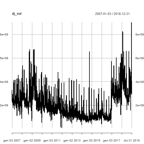
Now we want to identify and date such level shifts. First, we verify that a linear regression with constant mean is statistically significant.
lm_dj_vol <- lm(dj_vol ~ 1, data = dj_vol)
summary(lm_dj_vol)
##
## Call:
## lm(formula = dj_vol ~ 1, data = dj_vol)
##
## Residuals:
##        Min         1Q     Median         3Q        Max
## -193537268  -91369768  -25727268   65320232  698562732
##
## Coefficients:
##              Estimate Std. Error t value Pr(>|t|)
## (Intercept) 201947268    2060772      98   <2e-16 ***
## ---
## Signif. codes:  0 '***' 0.001 '**' 0.01 '*' 0.05 '.' 0.1 ' ' 1
##
## Residual standard error: 113200000 on 3019 degrees of freedom
Such linear regression model is statistically significant, hence it makes sense to proceed on with the breakpoints structural identification with respect a constant value.
bp_dj_vol <- breakpoints(dj_vol ~ 1, h = 0.1)
summary(bp_dj_vol)
##
##   Optimal (m+1)-segment partition:
##
## Call:
## breakpoints.formula(formula = dj_vol ~ 1, h = 0.1)
##
## Breakpoints at observation number:
##
## m = 1                                   2499
## m = 2           896                     2499
## m = 3       626     1254                2499
## m = 4   342 644     1254                2499
## m = 5   342 644     1219 1649           2499
## m = 6   320 622 924 1251 1649           2499
## m = 7   320 622 924 1251 1692      2172 2499
## m = 8   320 622 924 1251 1561 1863 2172 2499
##
## Corresponding to breakdates:
##
## m = 1
## m = 2                                       0.296688741721854
## m = 3                     0.207284768211921
## m = 4   0.113245033112583 0.213245033112583
## m = 5   0.113245033112583 0.213245033112583
## m = 6   0.105960264900662 0.205960264900662 0.305960264900662
## m = 7   0.105960264900662 0.205960264900662 0.305960264900662
## m = 8   0.105960264900662 0.205960264900662 0.305960264900662
##
## m = 1
## m = 2
## m = 3   0.41523178807947
## m = 4   0.41523178807947
## m = 5   0.40364238410596  0.546026490066225
## m = 6   0.414238410596027 0.546026490066225
## m = 7   0.414238410596027 0.560264900662252
## m = 8   0.414238410596027 0.516887417218543 0.616887417218543
##
## m = 1                     0.827483443708609
## m = 2                     0.827483443708609
## m = 3                     0.827483443708609
## m = 4                     0.827483443708609
## m = 5                     0.827483443708609
## m = 6                     0.827483443708609
## m = 7   0.719205298013245 0.827483443708609
## m = 8   0.719205298013245 0.827483443708609
##
## Fit:
##
## m   0         1         2         3         4         5         6
## RSS 3.872e+19 2.772e+19 1.740e+19 1.547e+19 1.515e+19 1.490e+19 1.475e+19
## BIC 1.206e+05 1.196e+05 1.182e+05 1.179e+05 1.178e+05 1.178e+05 1.178e+05
##
## m   7         8
## RSS 1.472e+19 1.478e+19
## BIC 1.178e+05 1.178e+05
It gives this plot.
plot(bp_dj_vol)
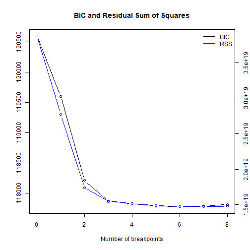
The minimum BIC is reached at breaks = 6.
Here is the plot of the DJIA daily trade volume with level shifts (red line).
bp_fit <- fitted(bp_dj_vol, breaks=6)
bp_fit_xts <- xts(bp_fit, order.by = index(dj_vol))
bb <- merge(bp_fit_xts, dj_vol)
colnames(bb) <- c("Level", "DJI.Volume")
plot(bb, lwd = c(3,1), col = c("red", "black"))
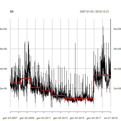
Here are the calendar dates when such level shifts occur.
bd <- breakdates(bp_dj_vol)
bd <- as.integer(nrow(dj_vol)*bd)
index(dj_vol)[bd]
## [1] "2008-04-10" "2009-06-22" "2010-09-01" "2011-12-16" "2013-07-22"
## [6] "2016-12-02"
See ref. [10] for further details about structural breaks.
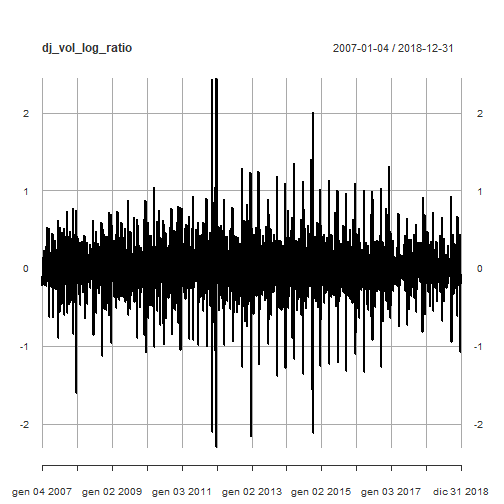
Daily Trade Volume Log Ratio Model
As shown in part 2, the daily trade volume log ratio:
\[
v_{t}\ := ln \frac{V_{t}}{V_{t-1}}
\]
is already available within our data environment. We plot it.
plot(dj_vol_log_ratio)
Outliers Detection
The Return.clean function within Performance Analytics package is able to clean return time series from outliers. Here below we compare the original time series with the outliers adjusted one.
dj_vol_log_ratio_outliersadj <- Return.clean(dj_vol_log_ratio, "boudt")
p <- plot(dj_vol_log_ratio)
p <- addSeries(dj_vol_log_ratio_outliersadj, col = 'blue', on = 1)
p
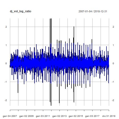
The prosecution of the analysis will be carried on with the original time series as a more conservative approach to volatility evaluation.
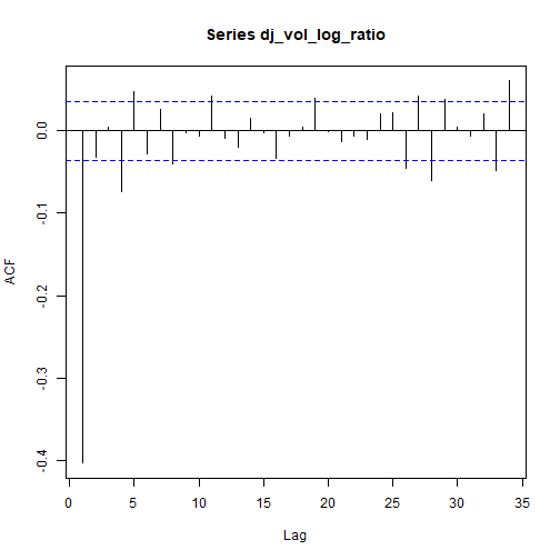
Correlation plots
Here below are the total and partial correlation plots.
acf(dj_vol_log_ratio)
pacf(dj_vol_log_ratio)
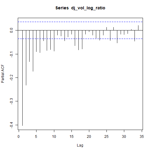
Above plots may suggest some ARMA(p,q) model with p and q > 0. That will be verified within the prosecution of the present analysis.
Unit root tests
We run the Augmented Dickey-Fuller test as available within the urca package. The no trend and no drift test flavor is run.
(urdftest_lag = floor(12* (nrow(dj_vol_log_ratio)/100)^0.25))
## [1] 28
summary(ur.df(dj_vol_log_ratio, type = "none", lags = urdftest_lag, selectlags="BIC"))
##
## ###############################################
## # Augmented Dickey-Fuller Test Unit Root Test #
## ###############################################
##
## Test regression none
##
##
## Call:
## lm(formula = z.diff ~ z.lag.1 - 1 + z.diff.lag)
##
## Residuals:
##      Min       1Q   Median       3Q      Max
## -2.51742 -0.13544 -0.02485  0.12006  1.98641
##
## Coefficients:
##              Estimate Std. Error t value Pr(>|t|)
## z.lag.1      -5.21571    0.25218 -20.682  < 2e-16 ***
## z.diff.lag1   3.59929    0.24637  14.609  < 2e-16 ***
## z.diff.lag2   3.14516    0.23796  13.217  < 2e-16 ***
## z.diff.lag3   2.78234    0.22809  12.198  < 2e-16 ***
## z.diff.lag4   2.41745    0.21700  11.140  < 2e-16 ***
## z.diff.lag5   2.14179    0.20472  10.462  < 2e-16 ***
## z.diff.lag6   1.88354    0.19168   9.826  < 2e-16 ***
## z.diff.lag7   1.66394    0.17781   9.358  < 2e-16 ***
## z.diff.lag8   1.41657    0.16304   8.688  < 2e-16 ***
## z.diff.lag9   1.19354    0.14771   8.080 9.31e-16 ***
## z.diff.lag10  1.00374    0.13207   7.600 3.95e-14 ***
## z.diff.lag11  0.88134    0.11634   7.575 4.75e-14 ***
## z.diff.lag12  0.74946    0.10027   7.474 1.02e-13 ***
## z.diff.lag13  0.60798    0.08399   7.239 5.73e-13 ***
## z.diff.lag14  0.48367    0.06732   7.185 8.46e-13 ***
## z.diff.lag15  0.36278    0.05108   7.102 1.53e-12 ***
## z.diff.lag16  0.21128    0.03470   6.088 1.29e-09 ***
## z.diff.lag17  0.07911    0.01833   4.315 1.65e-05 ***
## ---
## Signif. codes:  0 '***' 0.001 '**' 0.01 '*' 0.05 '.' 0.1 ' ' 1
##
## Residual standard error: 0.2576 on 2972 degrees of freedom
## Multiple R-squared:  0.7476, Adjusted R-squared:  0.746
## F-statistic: 488.9 on 18 and 2972 DF,  p-value: < 2.2e-16
##
##
## Value of test-statistic is: -20.6822
##
## Critical values for test statistics:
##       1pct  5pct 10pct
## tau1 -2.58 -1.95 -1.62
Based on reported test statistics compared with critical values, we reject the null hypothesis of unit root presence. See ref. [6] for further details about the Augmented Dickey-Fuller test.
ARMA model
We now determine the ARMA structure of our time series in order to run the ARCH effects test on the resulting residuals. That is in agreement with what outlined in ref. [4] $4.3.
We take advantage of auto.arima() function within forecast package (ref. [7]) to have an idea of what ARMA model to start with.
(auto_model_1 <- auto.arima(dj_vol_log_ratio, stepwise=FALSE))
## Series: dj_vol_log_ratio
## ARIMA(3,0,2) with zero mean
##
## Coefficients:
##           ar1     ar2     ar3      ma1      ma2
##       -0.5266  0.3769  0.1459  -0.0896  -0.7812
## s.e.   0.0970  0.0401  0.0203   0.0968   0.0872
##
## sigma^2 estimated as 0.0659:  log likelihood=-176.48
## AIC=364.96   AICc=364.99   BIC=401.03
coeftest(auto_model_1)
##
## z test of coefficients:
##
##      Estimate Std. Error z value  Pr(>|z|)
## ar1 -0.526617   0.096988 -5.4297 5.644e-08 ***
## ar2  0.376906   0.040090  9.4014 < 2.2e-16 ***
## ar3  0.145902   0.020324  7.1787 7.039e-13 ***
## ma1 -0.089611   0.096788 -0.9258    0.3545
## ma2 -0.781163   0.087159 -8.9626 < 2.2e-16 ***
## ---
## Signif. codes:  0 '***' 0.001 '**' 0.01 '*' 0.05 '.' 0.1 ' ' 1
The ma1 coefficient is not statistically significant. Hence we try with the following ARMA(2,3) model.
(arma_model_2 <- arima(dj_vol_log_ratio, order=c(2,0,3), include.mean = FALSE))
##
## Call:
## arima(x = dj_vol_log_ratio, order = c(2, 0, 3), include.mean = FALSE)
##
## Coefficients:
##           ar1     ar2      ma1      ma2     ma3
##       -0.1802  0.6441  -0.4351  -0.8604  0.3596
## s.e.   0.0643  0.0454   0.0681   0.0493  0.0423
##
## sigma^2 estimated as 0.0658:  log likelihood = -176.9,  aic = 363.79
coeftest(arma_model_2)
##
## z test of coefficients:
##
##      Estimate Std. Error  z value  Pr(>|z|)
## ar1 -0.180233   0.064315  -2.8023  0.005073 **
## ar2  0.644104   0.045449  14.1721 < 2.2e-16 ***
## ma1 -0.435122   0.068126  -6.3870 1.692e-10 ***
## ma2 -0.860443   0.049282 -17.4595 < 2.2e-16 ***
## ma3  0.359564   0.042307   8.4990 < 2.2e-16 ***
## ---
## Signif. codes:  0 '***' 0.001 '**' 0.01 '*' 0.05 '.' 0.1 ' ' 1
All coefficients are statistically significant and AIC is lower than the one of the first model. We then try with ARMA(1,2).
(arma_model_3 <- arima(dj_vol_log_ratio, order=c(1,0,2), include.mean = FALSE))
##
## Call:
## arima(x = dj_vol_log_ratio, order = c(1, 0, 2), include.mean = FALSE)
##
## Coefficients:
##          ar1      ma1     ma2
##       0.6956  -1.3183  0.3550
## s.e.  0.0439   0.0518  0.0453
##
## sigma^2 estimated as 0.06598:  log likelihood = -180.92,  aic = 367.84
coeftest(arma_model_3)
##
## z test of coefficients:
##
##      Estimate Std. Error  z value  Pr(>|z|)
## ar1  0.695565   0.043874  15.8537 < 2.2e-16 ***
## ma1 -1.318284   0.051787 -25.4557 < 2.2e-16 ***
## ma2  0.355015   0.045277   7.8409 4.474e-15 ***
## ---
## Signif. codes:  0 '***' 0.001 '**' 0.01 '*' 0.05 '.' 0.1 ' ' 1
This model has the highest AIC among the set and all coefficients are statistically significant.
We can also have a try with the eacf() function within the TSA package as further verification.
eacf(dj_vol_log_ratio)
## AR/MA
##   0 1 2 3 4 5 6 7 8 9 10 11 12 13
## 0 x o o x x o o x o o x  o  o  o
## 1 x x o x o o o x o o x  o  o  o
## 2 x x x x o o o o o o x  o  o  o
## 3 x x x x o o o o o o x  o  o  o
## 4 x x x x x o o o o o x  o  o  o
## 5 x x x x o o o o o o o  o  o  o
## 6 x x x x x o x o o o o  o  o  o
## 7 x x x x x o o o o o o  o  o  o
The upper left triangle with “O” as a vertex seems to be located somehow within {(1,2),(2,2),(1,3),(2,3)}, which represents the set of potential (p,q) values according to eacf() function output. To remark that we prefer to consider parsimonious models, that is why we do not go too far as AR and MA orders.
We already verified ARMA models with (p,q) orders within the set {(3,2)(2,3)(1,2)}. Let us try {(2,2)(1,3)}
(arma_model_4 <- arima(dj_vol_log_ratio, order=c(2,0,2), include.mean = FALSE))
##
## Call:
## arima(x = dj_vol_log_ratio, order = c(2, 0, 2), include.mean = FALSE)
##
## Coefficients:
##          ar1      ar2      ma1     ma2
##       0.7174  -0.0096  -1.3395  0.3746
## s.e.  0.1374   0.0560   0.1361  0.1247
##
## sigma^2 estimated as 0.06598:  log likelihood = -180.9,  aic = 369.8
coeftest(arma_model_4)
##
## z test of coefficients:
##
##       Estimate Std. Error z value  Pr(>|z|)
## ar1  0.7173631  0.1374135  5.2205 1.785e-07 ***
## ar2 -0.0096263  0.0560077 -0.1719  0.863536
## ma1 -1.3394720  0.1361208 -9.8403 < 2.2e-16 ***
## ma2  0.3746317  0.1247117  3.0040  0.002665 **
## ---
## Signif. codes:  0 '***' 0.001 '**' 0.01 '*' 0.05 '.' 0.1 ' ' 1
The ar2 coefficient is not statistically significant.
(arma_model_5 <- arima(dj_vol_log_ratio, order=c(1,0,3), include.mean = FALSE))
##
## Call:
## arima(x = dj_vol_log_ratio, order = c(1, 0, 3), include.mean = FALSE)
##
## Coefficients:
##          ar1      ma1     ma2     ma3
##       0.7031  -1.3253  0.3563  0.0047
## s.e.  0.0657   0.0684  0.0458  0.0281
##
## sigma^2 estimated as 0.06598:  log likelihood = -180.9,  aic = 369.8
coeftest(arma_model_5)
##
## z test of coefficients:
##
##       Estimate Std. Error  z value  Pr(>|z|)
## ar1  0.7030934  0.0656902  10.7032 < 2.2e-16 ***
## ma1 -1.3253176  0.0683526 -19.3894 < 2.2e-16 ***
## ma2  0.3563425  0.0458436   7.7730 7.664e-15 ***
## ma3  0.0047019  0.0280798   0.1674     0.867
## ---
## Signif. codes:  0 '***' 0.001 '**' 0.01 '*' 0.05 '.' 0.1 ' ' 1
The ma3 coefficient is not statistically significant.
As a conclusion, we keep both ARMA(1,2) and ARMA(2,3) as tentative mean models. We can now proceed on with ARCH effect tests.
ARCH effect Test
If ARCH effects are statistically significant for the residuals of our time series, a GARCH model is required.
We test the candidate mean model ARMA(2,3).
resid_dj_vol_log_ratio <- residuals(arma_model_2)
ArchTest(resid_dj_vol_log_ratio - mean(resid_dj_vol_log_ratio))
##
##  ARCH LM-test; Null hypothesis: no ARCH effects
##
## data:  resid_dj_vol_log_ratio - mean(resid_dj_vol_log_ratio)
## Chi-squared = 78.359, df = 12, p-value = 8.476e-12
Based on reported p-value, we reject the null hypothesis of no ARCH effects.
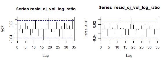
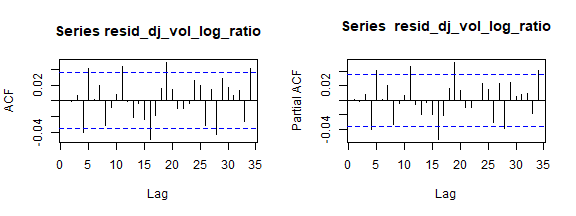
Let us have a look at the residual correlation plot too.
par(mfrow=c(1,2))
acf(resid_dj_vol_log_ratio)
pacf(resid_dj_vol_log_ratio)
We test the second candidate mean model, ARMA(1,2).
resid_dj_vol_log_ratio <- resid(arma_model_3)
ArchTest(resid_dj_vol_log_ratio - mean(resid_dj_vol_log_ratio))
##
##  ARCH LM-test; Null hypothesis: no ARCH effects
##
## data:  resid_dj_vol_log_ratio - mean(resid_dj_vol_log_ratio)
## Chi-squared = 74.768, df = 12, p-value = 4.065e-11
Based on reported p-value, we reject the null hypothesis of no ARCH effects.
Let us have a look at the residual correlation plots.
par(mfrow=c(1,2))
acf(resid_dj_vol_log_ratio)
pacf(resid_dj_vol_log_ratio)
To inspect asymmetries within the DJIA volume log ratio, summary statistics and density plot are shown.
basicStats(dj_vol_log_ratio)
##              DJI.Volume
## nobs        3019.000000
## NAs            0.000000
## Minimum       -2.301514
## Maximum        2.441882
## 1. Quartile   -0.137674
## 3. Quartile    0.136788
## Mean          -0.000041
## Median        -0.004158
## Sum           -0.124733
## SE Mean        0.005530
## LCL Mean      -0.010885
## UCL Mean       0.010802
## Variance       0.092337
## Stdev          0.303869
## Skewness      -0.182683
## Kurtosis       9.463384
Negative skewness is reported.
plot(density(dj_vol_log_ratio))
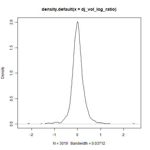
As a result, also for daily trade volume log ratio the eGARCH model will be proposed.
We run two fits in order to compare the results with two candidate mean models ARMA(1,2) and ARMA(2,3)
ARMA-GARCH: ARMA(1,2) + eGARCH(1,1)
garchspec <- ugarchspec(mean.model = list(armaOrder = c(1,2), include.mean = FALSE),
                        variance.model = list(model = "eGARCH", garchOrder = c(1, 1), variance.targeting = FALSE),
                        distribution.model = "sstd")

(garchfit <- ugarchfit(data = dj_vol_log_ratio, spec = garchspec, solver='hybrid'))
##
## *---------------------------------*
## *          GARCH Model Fit        *
## *---------------------------------*
##
## Conditional Variance Dynamics
## -----------------------------------
## GARCH Model  : eGARCH(1,1)
## Mean Model   : ARFIMA(1,0,2)
## Distribution : sstd
##
## Optimal Parameters
## ------------------------------------
##         Estimate  Std. Error     t value Pr(>|t|)
## ar1      0.67731    0.014856     45.5918  0.0e+00
## ma1     -1.22817    0.000038 -31975.1819  0.0e+00
## ma2      0.27070    0.000445    608.3525  0.0e+00
## omega   -1.79325    0.207588     -8.6385  0.0e+00
## alpha1   0.14348    0.032569      4.4053  1.1e-05
## beta1    0.35819    0.073164      4.8957  1.0e-06
## gamma1   0.41914    0.042252      9.9199  0.0e+00
## skew     1.32266    0.031528     41.9518  0.0e+00
## shape    3.54346    0.221750     15.9795  0.0e+00
##
## Robust Standard Errors:
##         Estimate  Std. Error     t value Pr(>|t|)
## ar1      0.67731    0.022072     30.6859  0.0e+00
## ma1     -1.22817    0.000067 -18466.0626  0.0e+00
## ma2      0.27070    0.000574    471.4391  0.0e+00
## omega   -1.79325    0.233210     -7.6894  0.0e+00
## alpha1   0.14348    0.030588      4.6906  3.0e-06
## beta1    0.35819    0.082956      4.3178  1.6e-05
## gamma1   0.41914    0.046728      8.9698  0.0e+00
## skew     1.32266    0.037586     35.1902  0.0e+00
## shape    3.54346    0.238225     14.8744  0.0e+00
##
## LogLikelihood : 347.9765
##
## Information Criteria
## ------------------------------------
##
## Akaike       -0.22456
## Bayes        -0.20664
## Shibata      -0.22458
## Hannan-Quinn -0.21812
##
## Weighted Ljung-Box Test on Standardized Residuals
## ------------------------------------
##                          statistic   p-value
## Lag[1]                      0.5812 4.459e-01
## Lag[2*(p+q)+(p+q)-1][8]     8.5925 3.969e-08
## Lag[4*(p+q)+(p+q)-1][14]   14.1511 4.171e-03
## d.o.f=3
## H0 : No serial correlation
##
## Weighted Ljung-Box Test on Standardized Squared Residuals
## ------------------------------------
##                         statistic p-value
## Lag[1]                     0.4995  0.4797
## Lag[2*(p+q)+(p+q)-1][5]    1.1855  0.8164
## Lag[4*(p+q)+(p+q)-1][9]    2.4090  0.8510
## d.o.f=2
##
## Weighted ARCH LM Tests
## ------------------------------------
##             Statistic Shape Scale P-Value
## ARCH Lag[3]    0.4215 0.500 2.000  0.5162
## ARCH Lag[5]    0.5974 1.440 1.667  0.8545
## ARCH Lag[7]    1.2835 2.315 1.543  0.8636
##
## Nyblom stability test
## ------------------------------------
## Joint Statistic:  5.2333
## Individual Statistics:
## ar1    0.63051
## ma1    1.18685
## ma2    1.11562
## omega  2.10211
## alpha1 0.08261
## beta1  2.07607
## gamma1 0.15883
## skew   0.33181
## shape  2.56140
##
## Asymptotic Critical Values (10% 5% 1%)
## Joint Statistic:          2.1 2.32 2.82
## Individual Statistic:     0.35 0.47 0.75
##
## Sign Bias Test
## ------------------------------------
##                    t-value    prob sig
## Sign Bias            1.600 0.10965
## Negative Sign Bias   0.602 0.54725
## Positive Sign Bias   2.540 0.01115  **
## Joint Effect         6.815 0.07804   *
##
##
## Adjusted Pearson Goodness-of-Fit Test:
## ------------------------------------
##   group statistic p-value(g-1)
## 1    20     20.37       0.3726
## 2    30     36.82       0.1510
## 3    40     45.07       0.2328
## 4    50     52.03       0.3567
##
##
## Elapsed time : 1.364722
All coefficients are statistically significant. However, based on above reported Weighted Ljung-Box Test on Standardized Residuals p-values, we reject the null hypothesis of no correlation of residuals for the present model. Hence model ARMA(1,2)+eGARCH(1,1) is not able to capture all the structure of our time series.
ARMA-GARCH: ARMA(2,3) + eGARCH(1,1)
garchspec <- ugarchspec(mean.model = list(armaOrder = c(2,3), include.mean = FALSE),
                        variance.model = list(model = "eGARCH", garchOrder = c(1, 1), variance.targeting = FALSE),
                        distribution.model = "sstd")

(garchfit <- ugarchfit(data = dj_vol_log_ratio, spec = garchspec, solver='hybrid'))
##
## *---------------------------------*
## *          GARCH Model Fit        *
## *---------------------------------*
##
## Conditional Variance Dynamics
## -----------------------------------
## GARCH Model  : eGARCH(1,1)
## Mean Model   : ARFIMA(2,0,3)
## Distribution : sstd
##
## Optimal Parameters
## ------------------------------------
##         Estimate  Std. Error   t value Pr(>|t|)
## ar1     -0.18607    0.008580  -21.6873  0.0e+00
## ar2      0.59559    0.004596  129.5884  0.0e+00
## ma1     -0.35619    0.013512  -26.3608  0.0e+00
## ma2     -0.83010    0.004689 -177.0331  0.0e+00
## ma3      0.26277    0.007285   36.0678  0.0e+00
## omega   -1.92262    0.226738   -8.4795  0.0e+00
## alpha1   0.14382    0.033920    4.2401  2.2e-05
## beta1    0.31060    0.079441    3.9098  9.2e-05
## gamma1   0.43137    0.043016   10.0281  0.0e+00
## skew     1.32282    0.031382   42.1523  0.0e+00
## shape    3.48939    0.220787   15.8043  0.0e+00
##
## Robust Standard Errors:
##         Estimate  Std. Error   t value Pr(>|t|)
## ar1     -0.18607    0.023940   -7.7724 0.000000
## ar2      0.59559    0.022231   26.7906 0.000000
## ma1     -0.35619    0.024244  -14.6918 0.000000
## ma2     -0.83010    0.004831 -171.8373 0.000000
## ma3      0.26277    0.030750    8.5453 0.000000
## omega   -1.92262    0.266462   -7.2154 0.000000
## alpha1   0.14382    0.032511    4.4239 0.000010
## beta1    0.31060    0.095329    3.2582 0.001121
## gamma1   0.43137    0.047092    9.1602 0.000000
## skew     1.32282    0.037663   35.1225 0.000000
## shape    3.48939    0.223470   15.6146 0.000000
##
## LogLikelihood : 356.4994
##
## Information Criteria
## ------------------------------------
##
## Akaike       -0.22888
## Bayes        -0.20698
## Shibata      -0.22891
## Hannan-Quinn -0.22101
##
## Weighted Ljung-Box Test on Standardized Residuals
## ------------------------------------
##                          statistic p-value
## Lag[1]                      0.7678 0.38091
## Lag[2*(p+q)+(p+q)-1][14]    7.7336 0.33963
## Lag[4*(p+q)+(p+q)-1][24]   17.1601 0.04972
## d.o.f=5
## H0 : No serial correlation
##
## Weighted Ljung-Box Test on Standardized Squared Residuals
## ------------------------------------
##                         statistic p-value
## Lag[1]                      0.526  0.4683
## Lag[2*(p+q)+(p+q)-1][5]     1.677  0.6965
## Lag[4*(p+q)+(p+q)-1][9]     2.954  0.7666
## d.o.f=2
##
## Weighted ARCH LM Tests
## ------------------------------------
##             Statistic Shape Scale P-Value
## ARCH Lag[3]     1.095 0.500 2.000  0.2955
## ARCH Lag[5]     1.281 1.440 1.667  0.6519
## ARCH Lag[7]     1.940 2.315 1.543  0.7301
##
## Nyblom stability test
## ------------------------------------
## Joint Statistic:  5.3764
## Individual Statistics:
## ar1    0.12923
## ar2    0.20878
## ma1    1.15005
## ma2    1.15356
## ma3    0.97487
## omega  2.04688
## alpha1 0.09695
## beta1  2.01026
## gamma1 0.18039
## skew   0.38131
## shape  2.40996
##
## Asymptotic Critical Values (10% 5% 1%)
## Joint Statistic:          2.49 2.75 3.27
## Individual Statistic:     0.35 0.47 0.75
##
## Sign Bias Test
## ------------------------------------
##                    t-value    prob sig
## Sign Bias           1.4929 0.13556
## Negative Sign Bias  0.6317 0.52766
## Positive Sign Bias  2.4505 0.01432  **
## Joint Effect        6.4063 0.09343   *
##
##
## Adjusted Pearson Goodness-of-Fit Test:
## ------------------------------------
##   group statistic p-value(g-1)
## 1    20     17.92       0.5278
## 2    30     33.99       0.2395
## 3    40     44.92       0.2378
## 4    50     50.28       0.4226
##
##
## Elapsed time : 1.660402
All coefficients are statistically significant. No correlation within standardized residuals or standardized squared residuals is found. All ARCH effects are properly captured by the model. The Adjusted Pearson Goodness-of-fit test does not reject the null hypothesis that the empirical distribution of the standardized residuals and the selected theoretical distribution are the same. However:
* the Nyblom stability test null hypothesis that the model parameters are constant over time is rejected for some of them
* the Positive Sign Bias null hypothesis is rejected at 5% of significance level; this kind of test focuses on the effect of large and small positive shocks
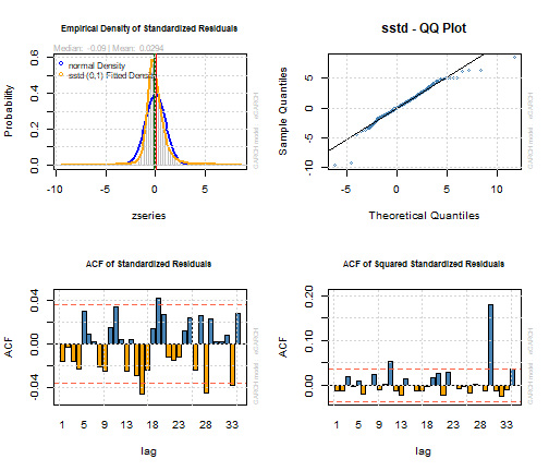
See ref. [11] for an explanation about GARCH model diagnostic.
Some diagnostic plots are shown.
par(mfrow=c(2,2))
plot(garchfit, which=8)
plot(garchfit, which=9)
plot(garchfit, which=10)
plot(garchfit, which=11)
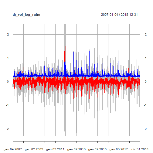
We show the original DJIA daily trade volume log ratio time series with the mean model fit (red line) and the conditional volatility (blue line).
par(mfrow=c(1,1))
cond_volatility <- sigma(garchfit)
mean_model_fit <- fitted(garchfit)
p <- plot(dj_vol_log_ratio, col = "grey")
p <- addSeries(mean_model_fit, col = 'red', on = 1)
p <- addSeries(cond_volatility, col = 'blue', on = 1)
p
Model Equation
Combining both ARMA(2,3) and eGARCH(1,1) model equations we have:
\[
\begin{equation}
\begin{cases}
y_{t}\ -\ \phi_{1}y_{t-1}\ -\ \phi_{2}y_{t-2} =\ \phi_{0}\ +\ u_{t}\ +\ \theta_{1}u_{t-1}\ +\ \theta_{2}u_{t-2}\ +\ \theta_{3}u_{t-3}
\\
\\
u_{t}\ =\ \sigma_{t}\epsilon_{t},\ \ \ \ \ \epsilon_{t}=N(0,1)
\\
\\
\ln(\sigma_{t}^2)\ =\ \omega\ + \sum_{j=1}^{q} (\alpha_{j} \epsilon_{t-j}^2\ + \gamma (\epsilon_{t-j} – E|\epsilon_{t-j}|)) +\ \sum_{i=1}^{p} \beta_{i} ln(\sigma_{t-1}^2)
\end{cases}
\end{equation}
\]
Using the model resulting coefficients we obtain:
\[
\begin{equation}
\begin{cases}
y_{t}\ +\ 0.186\ y_{t-1} -\ 0.595\ y_{t-2}\ = \ u_{t}\ -\ 0.356u_{t-1}\ – 0.830\ u_{t-2}\ +\ 0.263\ u_{t-3}
\\
\\
u_{t}\ =\ \sigma_{t}\epsilon_{t},\ \ \ \ \ \epsilon_{t}=N(0,1)
\\
\\
\ln(\sigma_{t}^2)\ =\ -1.922\ +0.144 \epsilon_{t-1}^2\ + 0.431\ (\epsilon_{t-1} – E|\epsilon_{t-1}|)) +\ 0.310\ ln(\sigma_{t-1}^2)
\end{cases}
\end{equation}
\]
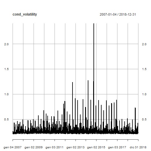
Daily Volume Log Ratio Volatility Analysis
Here is the plot of conditional volatility as resulting from our model ARMA(2,2)+eGARCH(1,1).
plot(cond_volatility)
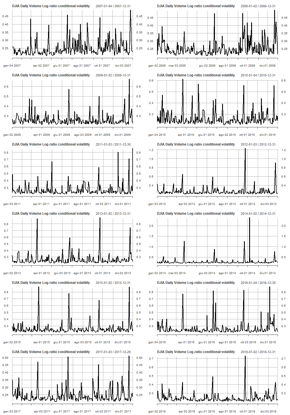
Line plots of conditional volatility by year are shown.
par(mfrow=c(6,2))
pl <- lapply(2007:2018, function(x) { plot(cond_volatility[as.character(x)], main = "DJIA Daily Volume Log-ratio conditional volatility")})
pl
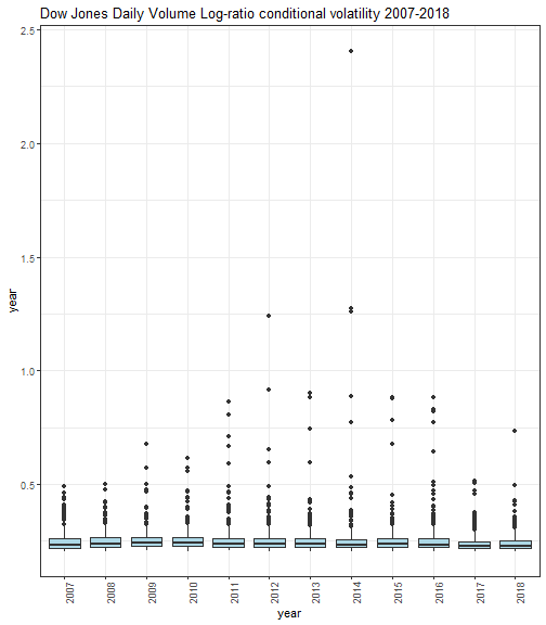
Conditional volatility box-plots by year are shown.
par(mfrow=c(1,1))
cond_volatility_df <- xts_to_dataframe(cond_volatility)
dataframe_boxplot(cond_volatility_df, "Dow Jones Daily Volume Log-ratio conditional volatility 2007-2018")
Conclusions
Resuming up what done within this post series.
We introduced summaries, line-plots and box-plots to highlight returns and trade volume changes over the years.
We investigated basic statistics metrics such as mean, meadian, skewness and kurtosis to understand how values are different over the years, also in terms of values distribution symmetries and tailedness. Starting from such summaries we obtained ordered lists of mean, median, skewness and kurtosis metrics to better highlight differences over years.
Box-plots allow to understand the statistics dispersion of the samples under analysis
Density plots allow to understand what are asymmetries and tailedness of our empirical samples distributions.
QQ plots highlight departures from normality. Such analysis is motivated by the need of understanding how close/far we are from the log-normal hypothesis assumed by some market models such as Black-Scholes one. If we have departures from normality, market models based under the log-normal distribution hypothesis might now work well.
For both log returns and volume log-ratio we built ARMA-GARCH models (exponential GARCH specifically as variance model), to obtain conditional volatility. Again, visualizations as line and box plots highlighted conditional volatility changes within and between years. Such kind of investigation is motivated by the fact that the volatility is an indicator of the amplitude of variations, to put it into simple words, and is a basic measure of risk when applied to log returns of an asset. There are several types of volatility (conditional, implied, realized volatility). See ref. 4 and 8 for details.
As explained in part 3, the conditional volatility at time t is the volatility of a random variable given the knowledge of hystorical data up to time t-1. To compute the conditional volatility, we have to build a GARCH model.
The trade volume may be interpreted as a measure of market activity magnitude and investors interest. To compute trade volume metrics (included volatility) gives an understanding of how such level of activity/interest changes over time.
If you have any questions, please feel free to comment below.
References
- Dow Jones Industrial Average
- Skewness ]
- Kurtosis ]
- An introduction to the analysis of financial data with R, Wiley, Ruey S. Tsay
- Time series analysis and its applications, Springer ed., R.H. Shumway, D.S. Stoffer
- Applied Econometric Time Series, Wiley, W. Enders, 4th ed.
- Forecasting – Principle and Practice, Texts, R.J. Hyndman
- Options, Futures and other Derivatives, Pearson ed., J.C. Hull
- An introduction to rugarch package
- Applied Econometrics with R, Achim Zeileis, Christian Kleiber – Springer Ed.
- GARCH modeling: diagnostic tests
Disclaimer
Any securities or databases referred in this post are solely for illustration purposes, and under no regard should the findings presented here be interpreted as investment advice or promotion of any particular security or source.
So, as this is the last part of your series, do you have any conclusions of your analysis?
I resumed up the basic steps.
Nice, thank you, but I was thinking of some economical conclusions 🙂
I understand that you do not want that “findings presented here must not be interpreted as investment advice”, but then what good does this mathematical analysis serve us? Then why we need to build GARCH model?
Ok, I will add such considerations to the “Conclusions” and post a reply when done.
I updated again adding some more details. Ref. 4 and 8 are the best ones to have a deep dive into such topics.