In this third post, I am going to build an ARMA-GARCH model for Dow Jones Industrial Average (DJIA) daily log-returns. You can read the first and second part which I published previously.
Packages
The packages being used in this post series are herein listed.
suppressPackageStartupMessages(library(lubridate))
suppressPackageStartupMessages(library(fBasics))
suppressPackageStartupMessages(library(lmtest))
suppressPackageStartupMessages(library(urca))
suppressPackageStartupMessages(library(ggplot2))
suppressPackageStartupMessages(library(quantmod))
suppressPackageStartupMessages(library(PerformanceAnalytics))
suppressPackageStartupMessages(library(rugarch))
suppressPackageStartupMessages(library(FinTS))
suppressPackageStartupMessages(library(forecast))
suppressPackageStartupMessages(library(strucchange))
suppressPackageStartupMessages(library(TSA))
Getting Data
We upload the environment status as saved at the end of part 2.
load(file='DowEnvironment.RData')
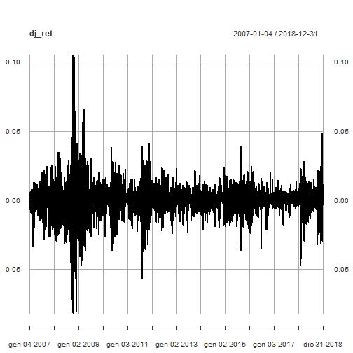
This is the plot of DJIA daily log-returns.
plot(dj_ret)
Outliers Detection
The Return.clean function within Performance Analytics package is able to clean return time series from outliers. Here below we compare the original time series with the outliers adjusted one.
dj_ret_outliersadj <- Return.clean(dj_ret, "boudt")
p <- plot(dj_ret)
p <- addSeries(dj_ret_outliersadj, col = 'blue', on = 1)
p
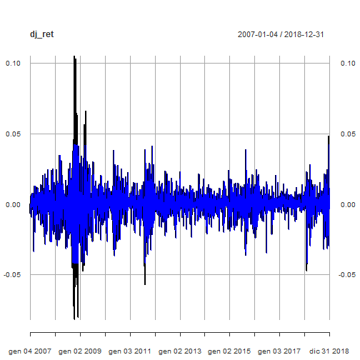
The prosecution of the analysis will be carried on with the original time series as a more conservative approach to volatility evaluation.
Correlation plots
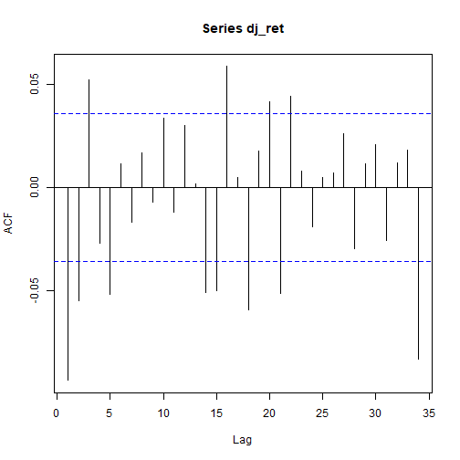
Here below are the total and partial correlation plots.
acf(dj_ret)
pacf(dj_ret)
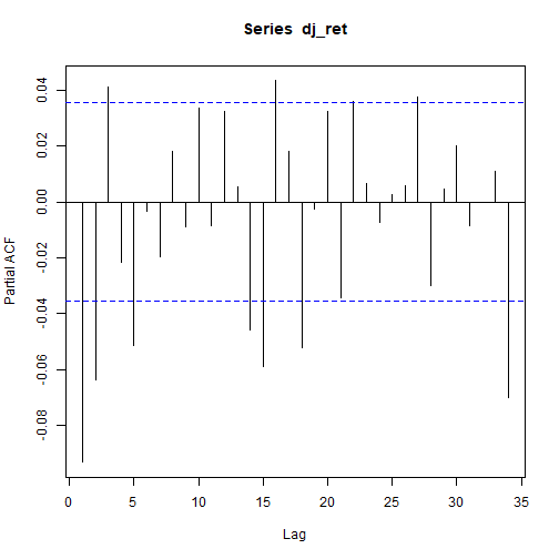
Above correlation plots suggest some ARMA(p,q) model with p and q > 0. That will be verified within the prosecution of the present analysis.
Unit root tests
We run the Augmented Dickey-Fuller test as available within the urca package. The no trend and no drift test flavor is run.
(urdftest_lag = floor(12* (nrow(dj_ret)/100)^0.25))
## [1] 28
summary(ur.df(dj_ret, type = "none", lags = urdftest_lag, selectlags="BIC"))
##
## ###############################################
## # Augmented Dickey-Fuller Test Unit Root Test #
## ###############################################
##
## Test regression none
##
##
## Call:
## lm(formula = z.diff ~ z.lag.1 - 1 + z.diff.lag)
##
## Residuals:
##       Min        1Q    Median        3Q       Max
## -0.081477 -0.004141  0.000762  0.005426  0.098777
##
## Coefficients:
##            Estimate Std. Error t value Pr(>|t|)
## z.lag.1    -1.16233    0.02699 -43.058  < 2e-16 ***
## z.diff.lag  0.06325    0.01826   3.464 0.000539 ***
## ---
## Signif. codes:  0 '***' 0.001 '**' 0.01 '*' 0.05 '.' 0.1 ' ' 1
##
## Residual standard error: 0.01157 on 2988 degrees of freedom
## Multiple R-squared:  0.5484, Adjusted R-squared:  0.5481
## F-statistic:  1814 on 2 and 2988 DF,  p-value: < 2.2e-16
##
##
## Value of test-statistic is: -43.0578
##
## Critical values for test statistics:
##       1pct  5pct 10pct
## tau1 -2.58 -1.95 -1.62
Based on reported test statistics compared with critical values, we reject the null hypothesis of unit root presence. See ref. [6] for further details about the Augmented Dickey-Fuller test.
ARMA model
We now determine the ARMA structure of our time series in order to run the ARCH effects test on the resulting residuals. That is in agreement with what outlined in ref. [4] $4.3.
ACF and PACF plots tailing off suggests an ARMA(2,2) (ref. [5], table $3.1). We take advantage of auto.arima() function within forecast package (ref. [7]) to have an idea to start with.
auto_model <- auto.arima(dj_ret)
summary(auto_model)
## Series: dj_ret
## ARIMA(2,0,4) with zero mean
##
## Coefficients:
##          ar1      ar2      ma1     ma2      ma3      ma4
##       0.4250  -0.8784  -0.5202  0.8705  -0.0335  -0.0769
## s.e.  0.0376   0.0628   0.0412  0.0672   0.0246   0.0203
##
## sigma^2 estimated as 0.0001322:  log likelihood=9201.19
## AIC=-18388.38   AICc=-18388.34   BIC=-18346.29
##
## Training set error measures:
##                        ME       RMSE         MAE MPE MAPE      MASE
## Training set 0.0002416895 0.01148496 0.007505056 NaN  Inf 0.6687536
##                      ACF1
## Training set -0.002537238
ARMA(2,4) model is suggested. However, the ma3 coefficient is not statistically significant, as further verified by:
coeftest(auto_model)
##
## z test of coefficients:
##
##      Estimate Std. Error  z value  Pr(>|z|)
## ar1  0.425015   0.037610  11.3007 < 2.2e-16 ***
## ar2 -0.878356   0.062839 -13.9779 < 2.2e-16 ***
## ma1 -0.520173   0.041217 -12.6204 < 2.2e-16 ***
## ma2  0.870457   0.067211  12.9511 < 2.2e-16 ***
## ma3 -0.033527   0.024641  -1.3606 0.1736335
## ma4 -0.076882   0.020273  -3.7923 0.0001492 ***
## ---
## Signif. codes:  0 '***' 0.001 '**' 0.01 '*' 0.05 '.' 0.1 ' ' 1
Hence we put as a constraint MA order q <= 2.
auto_model2 <- auto.arima(dj_ret, max.q=2)
summary(auto_model2)
## Series: dj_ret
## ARIMA(2,0,2) with zero mean
##
## Coefficients:
##           ar1      ar2     ma1     ma2
##       -0.5143  -0.4364  0.4212  0.3441
## s.e.   0.1461   0.1439  0.1512  0.1532
##
## sigma^2 estimated as 0.0001325:  log likelihood=9196.33
## AIC=-18382.66   AICc=-18382.64   BIC=-18352.6
##
## Training set error measures:
##                        ME       RMSE         MAE MPE MAPE      MASE
## Training set 0.0002287171 0.01150361 0.007501925 Inf  Inf 0.6684746
##                      ACF1
## Training set -0.002414944
Now all coefficients are statistically significant.
coeftest(auto_model2)
##
## z test of coefficients:
##
##     Estimate Std. Error z value  Pr(>|z|)
## ar1 -0.51428    0.14613 -3.5192 0.0004328 ***
## ar2 -0.43640    0.14392 -3.0322 0.0024276 **
## ma1  0.42116    0.15121  2.7853 0.0053485 **
## ma2  0.34414    0.15323  2.2458 0.0247139 *
## ---
## Signif. codes:  0 '***' 0.001 '**' 0.01 '*' 0.05 '.' 0.1 ' ' 1
Further verifications with ARMA(2,1) and ARMA(1,2) results with higher AIC values than ARMA(2,2). Hence ARMA(2,2) is preferable. Here are the results.
auto_model3 <- auto.arima(dj_ret, max.p=2, max.q=1)
summary(auto_model3)
## Series: dj_ret
## ARIMA(2,0,1) with zero mean
##
## Coefficients:
##           ar1      ar2     ma1
##       -0.4619  -0.1020  0.3646
## s.e.   0.1439   0.0204  0.1438
##
## sigma^2 estimated as 0.0001327:  log likelihood=9194.1
## AIC=-18380.2   AICc=-18380.19   BIC=-18356.15
##
## Training set error measures:
##                        ME       RMSE         MAE MPE MAPE      MASE
## Training set 0.0002370597 0.01151213 0.007522059 Inf  Inf 0.6702687
##                      ACF1
## Training set 0.0009366271
coeftest(auto_model3)
##
## z test of coefficients:
##
##      Estimate Std. Error z value  Pr(>|z|)
## ar1 -0.461916   0.143880 -3.2104  0.001325 **
## ar2 -0.102012   0.020377 -5.0062 5.552e-07 ***
## ma1  0.364628   0.143818  2.5353  0.011234 *
## ---
## Signif. codes:  0 '***' 0.001 '**' 0.01 '*' 0.05 '.' 0.1 ' ' 1
All coefficients are statistically significant.
auto_model4 <- auto.arima(dj_ret, max.p=1, max.q=2)
summary(auto_model4)
## Series: dj_ret
## ARIMA(1,0,2) with zero mean
##
## Coefficients:
##           ar1     ma1      ma2
##       -0.4207  0.3259  -0.0954
## s.e.   0.1488  0.1481   0.0198
##
## sigma^2 estimated as 0.0001328:  log likelihood=9193.01
## AIC=-18378.02   AICc=-18378   BIC=-18353.96
##
## Training set error measures:
##                        ME      RMSE         MAE MPE MAPE      MASE
## Training set 0.0002387398 0.0115163 0.007522913 Inf  Inf 0.6703448
##                      ACF1
## Training set -0.001958194
coeftest(auto_model4)
##
## z test of coefficients:
##
##      Estimate Std. Error z value  Pr(>|z|)
## ar1 -0.420678   0.148818 -2.8268  0.004702 **
## ma1  0.325918   0.148115  2.2004  0.027776 *
## ma2 -0.095407   0.019848 -4.8070 1.532e-06 ***
## ---
## Signif. codes:  0 '***' 0.001 '**' 0.01 '*' 0.05 '.' 0.1 ' ' 1
All coefficients are statistically significant.
Furthermore, we investigate what eacf() function within the TSA package reports.
eacf(dj_ret)
## AR/MA
##   0 1 2 3 4 5 6 7 8 9 10 11 12 13
## 0 x x x o x o o o o o o  o  o  x
## 1 x x o o x o o o o o o  o  o  o
## 2 x o o x x o o o o o o  o  o  o
## 3 x o x o x o o o o o o  o  o  o
## 4 x x x x x o o o o o o  o  o  o
## 5 x x x x x o o x o o o  o  o  o
## 6 x x x x x x o o o o o  o  o  o
## 7 x x x x x o o o o o o  o  o  o
The upper left triangle with “O” as a vertex seems to be located somehow within (p,q) = {(1,2),(2,2),(1,3)}, which represents a set of potential candidate (p,q) values according to eacf function output. To remark that we prefer to consider parsimoniuos models, that is why we do not go too far as AR and MA orders.
ARMA(1,2) model was already verified. ARMA(2,2) is already a candidate model. Let us verify ARMA(1,3).
(arima_model5 <- arima(dj_ret, order=c(1,0,3), include.mean = FALSE))
##
## Call:
## arima(x = dj_ret, order = c(1, 0, 3), include.mean = FALSE)
##
## Coefficients:
##           ar1     ma1      ma2     ma3
##       -0.2057  0.1106  -0.0681  0.0338
## s.e.   0.2012  0.2005   0.0263  0.0215
##
## sigma^2 estimated as 0.0001325:  log likelihood = 9193.97,  aic = -18379.94
coeftest(arima_model5)
##
## z test of coefficients:
##
##      Estimate Std. Error z value Pr(>|z|)
## ar1 -0.205742   0.201180 -1.0227 0.306461
## ma1  0.110599   0.200475  0.5517 0.581167
## ma2 -0.068124   0.026321 -2.5882 0.009647 **
## ma3  0.033832   0.021495  1.5739 0.115501
## ---
## Signif. codes:  0 '***' 0.001 '**' 0.01 '*' 0.05 '.' 0.1 ' ' 1
Only one coefficient is statistically significant.
As a conclusion, we choose ARMA(2,2) as mean model. We can now proceed on with ARCH effect tests.
ARCH effect test
Now, we can test if any ARCH effects are present on residuals of our model. If ARCH effects are statistically significant for the residuals of our time series, a GARCH model is required.
model_residuals <- residuals(auto_model2)
ArchTest(model_residuals - mean(model_residuals))
##
##  ARCH LM-test; Null hypothesis: no ARCH effects
##
## data:  model_residuals - mean(model_residuals)
## Chi-squared = 986.82, df = 12, p-value < 2.2e-16
Based on reported p-value, we reject the null hypothesis of no ARCH effects.
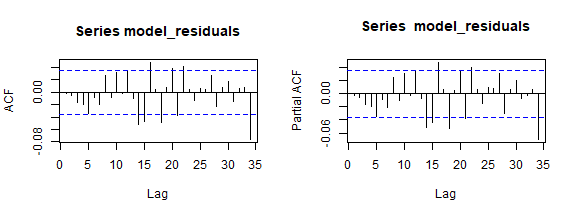
Let us have a look at the residual correlation plots.
par(mfrow=c(1,2))
acf(model_residuals)
pacf(model_residuals)
Conditional Volatility
The conditional mean and variance are defined as:
\[
\mu_{t}\ :=\ E(r_{t}|\ F_{t-1}) \\
\sigma^2_{t}\ :=\ Var(r_{t}|\ F_{t-1})\ =\ E[(r_t-\mu_{t})^2| F_{t-1}]
\]
The conditional volatility can be computed as square root of the conditional variance. See ref. [4] for further details.
eGARCH Model
The attempts with sGARCH as variance model did not bring to result with statistically significant coefficients. On the contrary, the exponential GARCH (eGARCH) variance model is capable to capture asymmetries within the volatility shocks.
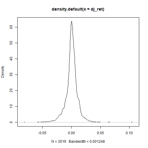
To inspect asymmetries within the DJIA log returns, summary statistics and density plot are shown.
basicStats(dj_ret)
##             DJI.Adjusted
## nobs         3019.000000
## NAs             0.000000
## Minimum        -0.082005
## Maximum         0.105083
## 1. Quartile    -0.003991
## 3. Quartile     0.005232
## Mean            0.000207
## Median          0.000551
## Sum             0.625943
## SE Mean         0.000211
## LCL Mean       -0.000206
## UCL Mean        0.000621
## Variance        0.000134
## Stdev           0.011593
## Skewness       -0.141370
## Kurtosis       10.200492
The negative skewness value confirms the presence of asymmetries within the DJIA distribution.
This gives the density plot.
plot(density(dj_ret))
We go on proposing as variance model (for conditional variance) the eGARCH model. More precisely, we are about to model an ARMA-GARCH, with ARMA(2,2) as a mean model and exponential GARCH(1,1) as the variance model. Before doing that, we further emphasize how ARMA(0,0) is not satisfactory within this context.
ARMA-GARCH: ARMA(0,0) + eGARCH(1,1)
garchspec <- ugarchspec(mean.model = list(armaOrder = c(0,0), include.mean = TRUE),
                        variance.model = list(model = "eGARCH", garchOrder = c(1, 1)),
                        distribution.model = "sstd")

(garchfit <- ugarchfit(data = dj_ret, spec = garchspec))
##
## *---------------------------------*
## *          GARCH Model Fit        *
## *---------------------------------*
##
## Conditional Variance Dynamics
## -----------------------------------
## GARCH Model  : eGARCH(1,1)
## Mean Model   : ARFIMA(0,0,0)
## Distribution : sstd
##
## Optimal Parameters
## ------------------------------------
##         Estimate  Std. Error  t value Pr(>|t|)
## mu      0.000303    0.000117   2.5933 0.009506
## omega  -0.291302    0.016580 -17.5699 0.000000
## alpha1 -0.174456    0.013913 -12.5387 0.000000
## beta1   0.969255    0.001770 547.6539 0.000000
## gamma1  0.188918    0.021771   8.6773 0.000000
## skew    0.870191    0.021763  39.9848 0.000000
## shape   6.118380    0.750114   8.1566 0.000000
##
## Robust Standard Errors:
##         Estimate  Std. Error  t value Pr(>|t|)
## mu      0.000303    0.000130   2.3253 0.020055
## omega  -0.291302    0.014819 -19.6569 0.000000
## alpha1 -0.174456    0.016852 -10.3524 0.000000
## beta1   0.969255    0.001629 595.0143 0.000000
## gamma1  0.188918    0.031453   6.0063 0.000000
## skew    0.870191    0.022733  38.2783 0.000000
## shape   6.118380    0.834724   7.3298 0.000000
##
## LogLikelihood : 10138.63
##
## Information Criteria
## ------------------------------------
##
## Akaike       -6.7119
## Bayes        -6.6980
## Shibata      -6.7119
## Hannan-Quinn -6.7069
##
## Weighted Ljung-Box Test on Standardized Residuals
## ------------------------------------
##                         statistic p-value
## Lag[1]                      5.475 0.01929
## Lag[2*(p+q)+(p+q)-1][2]     6.011 0.02185
## Lag[4*(p+q)+(p+q)-1][5]     7.712 0.03472
## d.o.f=0
## H0 : No serial correlation
##
## Weighted Ljung-Box Test on Standardized Squared Residuals
## ------------------------------------
##                         statistic p-value
## Lag[1]                      1.342  0.2467
## Lag[2*(p+q)+(p+q)-1][5]     2.325  0.5438
## Lag[4*(p+q)+(p+q)-1][9]     2.971  0.7638
## d.o.f=2
##
## Weighted ARCH LM Tests
## ------------------------------------
##             Statistic Shape Scale P-Value
## ARCH Lag[3]    0.3229 0.500 2.000  0.5699
## ARCH Lag[5]    1.4809 1.440 1.667  0.5973
## ARCH Lag[7]    1.6994 2.315 1.543  0.7806
##
## Nyblom stability test
## ------------------------------------
## Joint Statistic:  4.0468
## Individual Statistics:
## mu     0.2156
## omega  1.0830
## alpha1 0.5748
## beta1  0.8663
## gamma1 0.3994
## skew   0.1044
## shape  0.4940
##
## Asymptotic Critical Values (10% 5% 1%)
## Joint Statistic:          1.69 1.9 2.35
## Individual Statistic:     0.35 0.47 0.75
##
## Sign Bias Test
## ------------------------------------
##                    t-value    prob sig
## Sign Bias            1.183 0.23680
## Negative Sign Bias   2.180 0.02932  **
## Positive Sign Bias   1.554 0.12022
## Joint Effect         8.498 0.03677  **
##
##
## Adjusted Pearson Goodness-of-Fit Test:
## ------------------------------------
##   group statistic p-value(g-1)
## 1    20     37.24      0.00741
## 2    30     42.92      0.04633
## 3    40     52.86      0.06831
## 4    50     65.55      0.05714
##
##
## Elapsed time : 0.6527421
All coefficients are statistically significant. However, from Weighted Ljung-Box Test on Standardized Residuals reported p-value above (as part of the overall report), we have the confirmation that such model does not capture all the structure (we reject the null hypothesis of no correlation within the residuals).
As a conclusion, we proceed on by specifying ARMA(2,2) as a mean model within our GARCH fit as hereinbelow shown.
ARMA-GARCH: ARMA(2,2) + eGARCH(1,1)
garchspec <- ugarchspec(mean.model = list(armaOrder = c(2,2), include.mean = FALSE),
                        variance.model = list(model = "eGARCH", garchOrder = c(1, 1)),
                        distribution.model = "sstd")

(garchfit <- ugarchfit(data = dj_ret, spec = garchspec))
##
## *---------------------------------*
## *          GARCH Model Fit        *
## *---------------------------------*
##
## Conditional Variance Dynamics
## -----------------------------------
## GARCH Model  : eGARCH(1,1)
## Mean Model   : ARFIMA(2,0,2)
## Distribution : sstd
##
## Optimal Parameters
## ------------------------------------
##         Estimate  Std. Error    t value Pr(>|t|)
## ar1     -0.47642    0.026115   -18.2433        0
## ar2     -0.57465    0.052469   -10.9523        0
## ma1      0.42945    0.025846    16.6157        0
## ma2      0.56258    0.054060    10.4066        0
## omega   -0.31340    0.003497   -89.6286        0
## alpha1  -0.17372    0.011642   -14.9222        0
## beta1    0.96598    0.000027 35240.1590        0
## gamma1   0.18937    0.011893    15.9222        0
## skew     0.84959    0.020063    42.3469        0
## shape    5.99161    0.701313     8.5434        0
##
## Robust Standard Errors:
##         Estimate  Std. Error    t value Pr(>|t|)
## ar1     -0.47642    0.007708   -61.8064        0
## ar2     -0.57465    0.018561   -30.9608        0
## ma1      0.42945    0.007927    54.1760        0
## ma2      0.56258    0.017799    31.6074        0
## omega   -0.31340    0.003263   -96.0543        0
## alpha1  -0.17372    0.012630   -13.7547        0
## beta1    0.96598    0.000036 26838.0412        0
## gamma1   0.18937    0.013003    14.5631        0
## skew     0.84959    0.020089    42.2911        0
## shape    5.99161    0.707324     8.4708        0
##
## LogLikelihood : 10140.27
##
## Information Criteria
## ------------------------------------
##
## Akaike       -6.7110
## Bayes        -6.6911
## Shibata      -6.7110
## Hannan-Quinn -6.7039
##
## Weighted Ljung-Box Test on Standardized Residuals
## ------------------------------------
##                          statistic p-value
## Lag[1]                     0.03028  0.8619
## Lag[2*(p+q)+(p+q)-1][11]   5.69916  0.6822
## Lag[4*(p+q)+(p+q)-1][19]  12.14955  0.1782
## d.o.f=4
## H0 : No serial correlation
##
## Weighted Ljung-Box Test on Standardized Squared Residuals
## ------------------------------------
##                         statistic p-value
## Lag[1]                      1.666  0.1967
## Lag[2*(p+q)+(p+q)-1][5]     2.815  0.4418
## Lag[4*(p+q)+(p+q)-1][9]     3.457  0.6818
## d.o.f=2
##
## Weighted ARCH LM Tests
## ------------------------------------
##             Statistic Shape Scale P-Value
## ARCH Lag[3]    0.1796 0.500 2.000  0.6717
## ARCH Lag[5]    1.5392 1.440 1.667  0.5821
## ARCH Lag[7]    1.6381 2.315 1.543  0.7933
##
## Nyblom stability test
## ------------------------------------
## Joint Statistic:  4.4743
## Individual Statistics:
## ar1    0.07045
## ar2    0.37070
## ma1    0.07702
## ma2    0.39283
## omega  1.00123
## alpha1 0.49520
## beta1  0.79702
## gamma1 0.51601
## skew   0.07163
## shape  0.55625
##
## Asymptotic Critical Values (10% 5% 1%)
## Joint Statistic:          2.29 2.54 3.05
## Individual Statistic:     0.35 0.47 0.75
##
## Sign Bias Test
## ------------------------------------
##                    t-value    prob sig
## Sign Bias           0.4723 0.63677
## Negative Sign Bias  1.7969 0.07246   *
## Positive Sign Bias  2.0114 0.04438  **
## Joint Effect        7.7269 0.05201   *
##
##
## Adjusted Pearson Goodness-of-Fit Test:
## ------------------------------------
##   group statistic p-value(g-1)
## 1    20     46.18    0.0004673
## 2    30     47.73    0.0156837
## 3    40     67.07    0.0034331
## 4    50     65.51    0.0574582
##
##
## Elapsed time : 0.93679
All coefficients are statistically significant. No correlation within standardized residuals or standardized squared residuals is found. All ARCH effects are properly captured by the model. However:
* the Nyblom stability test null hypothesis that the model parameters are constant over time is rejected for some of them
* the Positive Sign Bias null hypothesis is rejected at 5% level of significance; this kind of test focuses on the effect of large and small positive shocks
* the Adjusted Pearson Goodness-of-fit test null hypothesis that the empirical and theoretical distribution of standardized residuals are identical is rejected
See ref. [11] for an explanation about GARCH model diagnostic.
Note: The ARMA(1,2) + eGARCH(1,1) fit also provides with statistically significant coefficients, no correlation within standardized residuals, no correlation within standardized squared residuals and all ARCH effects are properly captured. However the bias tests are less satisfactory at 5% than the ARMA(2,2) + eGARCH(1,1) model ones.
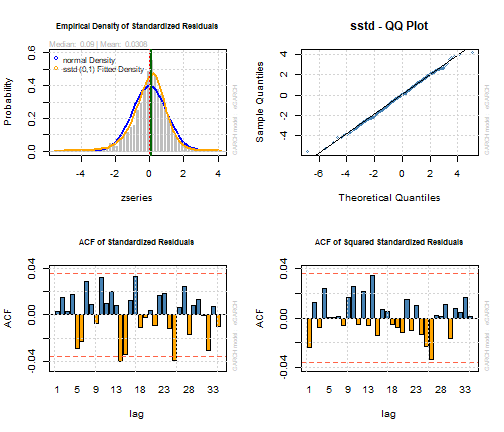
We show some diagnostic plots further.
par(mfrow=c(2,2))
plot(garchfit, which=8)
plot(garchfit, which=9)
plot(garchfit, which=10)
plot(garchfit, which=11)
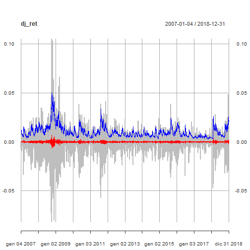
We show the original DJIA log-returns time series with the mean model fit (red line) and the conditional volatility (blue line).
par(mfrow=c(1,1))
cond_volatility <- sigma(garchfit)
mean_model_fit <- fitted(garchfit)
p <- plot(dj_ret, col = "grey")
p <- addSeries(mean_model_fit, col = 'red', on = 1)
p <- addSeries(cond_volatility, col = 'blue', on = 1)
p
Model Equation
Combining both ARMA(2,2) and eGARCH models we have:
\[
\begin{equation}
\begin{cases}
y_{t}\ -\ \phi_{1}y_{t-1}\ -\ \phi_{2}y_{t-2} =\ \phi_{0}\ +\ u_{t}\ +\ \theta_{1}u_{t-1}\ +\ \theta_{2}u_{t-2}
\\
\\
u_{t}\ =\ \sigma_{t}\epsilon_{t},\ \ \ \ \ \epsilon_{t}=N(0,1)
\\
\\
\ln(\sigma_{t}^2)\ =\ \omega\ + \sum_{j=1}^{q} (\alpha_{j} \epsilon_{t-j}^2\ + \gamma (\epsilon_{t-j} – E|\epsilon_{t-j}|)) +\ \sum_{i=1}^{p} \beta_{i} ln(\sigma_{t-1}^2)
\end{cases}
\end{equation}
\]
Using the model resulting coefficients, it results as follows.
\[
\begin{equation}
\begin{cases}
y_{t}\ + 0.476\ y_{t-1}\ + 0.575\ y_{t-2} = \ u_{t}\ + 0.429\ u_{t-1}\ + 0.563\ u_{t-2}
\\
\\
u_{t}\ =\ \sigma_{t}\epsilon_{t},\ \ \ \ \ \epsilon_{t}=N(0,1)
\\
\\
\ln(\sigma_{t}^2)\ =\ -0.313\ -0.174 \epsilon_{t-1}^2\ + 0.189\ (\epsilon_{t-1} – E|\epsilon_{t-1}|)) +\ 0.966\ ln(\sigma_{t-1}^2)
\end{cases}
\end{equation}
\]
Volatility Analysis
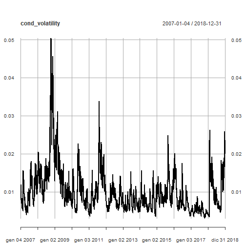
Here is the plot of conditional volatility as resulting from our ARMA(2,2) + eGARCH(1,1) model.
plot(cond_volatility)
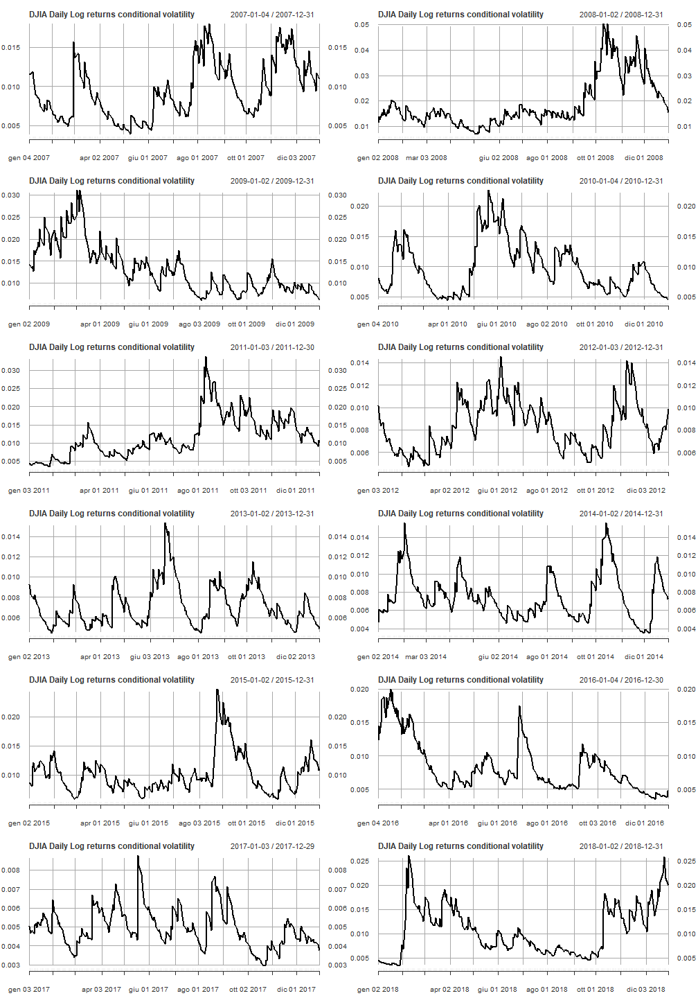
Line plots of conditional volatility by year are shown.
par(mfrow=c(6,2))
pl <- lapply(2007:2018, function(x) { plot(cond_volatility[as.character(x)], main = "DJIA Daily Log returns conditional volatility")})
pl
Conditional volatility box-plots by year are shown.
par(mfrow=c(1,1))
cond_volatility_df <- xts_to_dataframe(cond_volatility)
dataframe_boxplot(cond_volatility_df, "Dow Jones Daily Log-returns conditional Volatility 2007-2018")
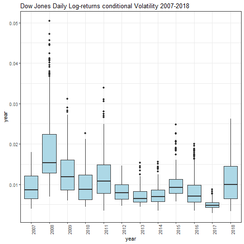
Afterwards 2008, the daily volatility basically tends to decrease. In the year 2017, the volatility was lower with respect any other year under analysis. Differently, on year 2018, we experienced a remarkable increase of volatility with respect year 2017.
Saving the current enviroment for further analysis.
save.image(file='DowEnvironment.RData')
If you have any questions, please feel free to comment below.
References
- Dow Jones Industrial Average
- Skewness
- Kurtosis
- An introduction to analysis of financial data with R, Wiley, Ruey S. Tsay
- Time series analysis and its applications, Springer ed., R.H. Shumway, D.S. Stoffer
- Applied Econometric Time Series, Wiley, W. Enders, 4th ed.
- Forecasting – Principle and Practice, Texts, R.J. Hyndman
- Options, Futures and other Derivatives, Pearson ed., J.C. Hull
- An introduction to rugarch package
- Applied Econometrics with R, Achim Zeileis, Christian Kleiber – Springer Ed.
- GARCH modeling: diagnostic tests
Disclaimer
Any securities or databases referred in this post are solely for illustration purposes, and under no regard should the findings presented here be interpreted as investment advice or promotion of any particular security or source.