In this post series, we are going to introduce the exploratory analysis of a dataset as available at ref. [1] reporting earthquakes and similar events occurring within a specific time window. We will run a basic exploratory analysis, showing some of the main principles and tools on that matter. Then, we will show how to represent the earthquakes dataset content on a geographical map, of static, interactive or animated flavor. Finally, a cluster analysis of earthquakes located onto specific geographical regions will be introduced. This post series is so organized:
- First post: exploratory analysis of quantitative variables.
- Second post: exploratory analysis of categorical variables.
- Third post: static, interactive and animated maps.
- Fourth post: cluster analysis.
Packages
Within the present post, I am going to take advantage of the following packages.
suppressPackageStartupMessages(library(ggplot2))
suppressPackageStartupMessages(library(ggmap))
suppressPackageStartupMessages(library(dplyr))
suppressPackageStartupMessages(library(factoextra))
suppressPackageStartupMessages(library(Hmisc))
suppressPackageStartupMessages(library(gridExtra))
suppressPackageStartupMessages(library(lubridate))
suppressPackageStartupMessages(library(corrplot))
suppressPackageStartupMessages(library(vcd))
suppressPackageStartupMessages(library(gmodels))
Packages versions are herein listed.
packages <- c("ggplot2", "ggmap", "dplyr", "factoextra", "Hmisc", "gridExtra", "lubridate", "corrplot", "vcd", "gmodels")
version <- lapply(packages, packageVersion)
version_c <- do.call(c, version)
data.frame(packages=packages, version = as.character(version_c))
##      packages version
## 1     ggplot2   3.1.0
## 2       ggmap   3.0.0
## 3       dplyr 0.8.0.1
## 4  factoextra   1.0.5
## 5       Hmisc   4.2.0
## 6   gridExtra     2.3
## 7   lubridate   1.7.4
## 8    corrplot    0.84
## 9         vcd   1.4.4
## 10    gmodels  2.18.1
Running on Windows-10 the following R language version.
R.version
##                _
## platform       x86_64-w64-mingw32
## arch           x86_64
## os             mingw32
## system         x86_64, mingw32
## status
## major          3
## minor          5.2
## year           2018
## month          12
## day            20
## svn rev        75870
## language       R
## version.string R version 3.5.2 (2018-12-20)
## nickname       Eggshell Igloo
Getting Data
We download the earthquake dataset from earthquake.usgs.gov, specifically the last 30 days dataset. Please note that such eartquake dataset is day by day updated to cover the last 30 days of data collection. If not already present into our workspace, we download and save it to be loaded into the quakes local variable. Please notice that it is not the most recent dataset available, as I collected it some weeks ago.
if ("all_week.csv" %in% dir(".") == FALSE) {
  url <- "https://earthquake.usgs.gov/earthquakes/feed/v1.0/summary/all_month.csv"
  download.file(url = url, destfile = "all_week.csv")
}
quakes <- read.csv("all_month.csv", header=TRUE, sep=',', stringsAsFactors = FALSE)
Dates and factors are so determined.
quakes$time <- ymd_hms(quakes$time)
quakes$updated <- ymd_hms(quakes$updated)
quakes$magType <- as.factor(quakes$magType)
quakes$net <- as.factor(quakes$net)
quakes$type <- as.factor(quakes$type)
quakes$status <- as.factor(quakes$status)
quakes$locationSource <- as.factor(quakes$locationSource)
quakes$magSource <- as.factor(quakes$magSource)
Number of rows and columns of our dataset are as shown.
dim(quakes)
## [1] 8407   22
We arrange rows in reverse order with respect the original, in order to have entries in incresing date ordering.
quakes <- arrange(quakes, -row_number())
The rows not having any missing values are:
sum(complete.cases(quakes))
## [1] 3957
That is a fraction wih respect the total number of records equal to:
sum(complete.cases(quakes))/nrow(quakes)
## [1] 0.4706792
Let us have a look at the data.
head(quakes)
##                  time latitude longitude depth  mag magType nst gap
## 1 2019-02-14 16:35:36  53.1050 -164.7006 20.20 2.30      ml  NA  NA
## 2 2019-02-14 16:42:10  33.5345 -116.7100  2.46 1.52      ml  37  35
## 3 2019-02-14 16:52:34  19.2010 -155.5120 34.29 2.34      ml  57  81
## 4 2019-02-14 17:00:44  60.5937 -147.8132 13.20 2.10      ml  NA  NA
## 5 2019-02-14 17:02:05  64.3332 -148.4033 11.50 0.90      ml  NA  NA
## 6 2019-02-14 17:06:09  65.4253 -153.3378 14.10 1.00      ml  NA  NA
##      dmin  rms net           id             updated
## 1      NA 0.30  ak ak01922ox4si 2019-03-01 21:51:59
## 2 0.03833 0.20  ci   ci37531042 2019-02-14 17:00:40
## 3 0.03755 0.09  hv   hv70811146 2019-02-14 19:21:24
## 4      NA 0.42  ak ak01922pb2w7 2019-03-01 21:51:36
## 5      NA 0.65  ak ak01922pbfay 2019-03-01 21:51:37
## 6      NA 0.83  ak ak01922pcak4 2019-03-01 21:52:00
##                             place       type horizontalError depthError
## 1     134km SSE of Akutan, Alaska earthquake              NA      27.00
## 2              4km SW of Anza, CA earthquake            0.22       0.26
## 3         3km W of Pahala, Hawaii earthquake            0.42       0.53
## 4    51km ESE of Whittier, Alaska earthquake              NA       0.20
## 5 43km SE of North Nenana, Alaska earthquake              NA       0.40
## 6      65km WNW of Tanana, Alaska earthquake              NA       0.10
##   magError magNst   status locationSource magSource
## 1       NA     NA reviewed             ak        ak
## 2    0.159     27 reviewed             ci        ci
## 3    0.177     21 reviewed             hv        hv
## 4       NA     NA reviewed             ak        ak
## 5       NA     NA reviewed             ak        ak
## 6       NA     NA reviewed             ak        ak
tail(quakes)
##                     time latitude longitude depth  mag magType nst gap
## 8402 2019-03-16 15:31:10 38.83517 -122.7977  2.24 0.56      md   7 106
## 8403 2019-03-16 15:33:11 37.60300 -121.6880 18.31 1.60      md  23  67
## 8404 2019-03-16 15:44:25 33.87533 -116.8533 11.28 0.93      ml  15  75
## 8405 2019-03-16 15:45:27 34.21200 -117.5643  8.40 2.27      ml  83  21
## 8406 2019-03-16 15:54:16 33.49667 -116.7853  2.56 0.44      ml  17  66
## 8407 2019-03-16 16:06:56 33.24683 -116.3273 14.15 2.86      ml  85  31
##          dmin  rms net         id             updated
## 8402 0.006573 0.01  nc nc73152836 2019-03-16 16:09:04
## 8403 0.058000 0.12  nc nc73152846 2019-03-16 16:20:03
## 8404 0.196700 0.19  ci ci38271511 2019-03-16 15:48:11
## 8405 0.053200 0.21  ci ci38271527 2019-03-16 15:56:41
## 8406 0.020070 0.19  ci ci38271535 2019-03-16 15:57:48
## 8407 0.272400 0.21  ci ci38271551 2019-03-16 16:19:48
##                               place       type horizontalError depthError
## 8402            7km WNW of Cobb, CA earthquake            0.50       1.47
## 8403       11km SE of Livermore, CA earthquake            0.36       0.54
## 8404         6km SSE of Banning, CA earthquake            0.35       1.47
## 8405      8km SW of Lytle Creek, CA earthquake            0.18       0.51
## 8406         10km NE of Aguanga, CA earthquake            0.35       0.41
## 8407 4km ESE of Borrego Springs, CA earthquake            0.19       0.55
##      magError magNst    status locationSource magSource
## 8402       NA      1 automatic             nc        nc
## 8403    0.110     11 automatic             nc        nc
## 8404    0.218     18 automatic             ci        ci
## 8405    0.159     24 automatic             ci        ci
## 8406    0.061     11 automatic             ci        ci
## 8407    0.151     25 automatic             ci        ci
The data structure is:
str(quakes)
## 'data.frame':    8407 obs. of  22 variables:
##  $ time           : POSIXct, format: "2019-02-14 16:35:36" "2019-02-14 16:42:10" ...
##  $ latitude       : num  53.1 33.5 19.2 60.6 64.3 ...
##  $ longitude      : num  -165 -117 -156 -148 -148 ...
##  $ depth          : num  20.2 2.46 34.29 13.2 11.5 ...
##  $ mag            : num  2.3 1.52 2.34 2.1 0.9 1 0.3 0.4 2.4 1.82 ...
##  $ magType        : Factor w/ 10 levels "","mb","mb_lg",..: 6 6 6 6 6 6 6 6 6 4 ...
##  $ nst            : int  NA 37 57 NA NA NA NA NA NA 5 ...
##  $ gap            : num  NA 35 81 NA NA NA NA NA NA 141 ...
##  $ dmin           : num  NA 0.0383 0.0376 NA NA ...
##  $ rms            : num  0.3 0.2 0.09 0.42 0.65 0.83 0.48 0.7 0.55 0.09 ...
##  $ net            : Factor w/ 14 levels "ak","ci","hv",..: 1 2 3 1 1 1 1 1 1 13 ...
##  $ id             : chr  "ak01922ox4si" "ci37531042" "hv70811146" "ak01922pb2w7" ...
##  $ updated        : POSIXct, format: "2019-03-01 21:51:59" "2019-02-14 17:00:40" ...
##  $ place          : chr  "134km SSE of Akutan, Alaska" "4km SW of Anza, CA" "3km W of Pahala, Hawaii" "51km ESE of Whittier, Alaska" ...
##  $ type           : Factor w/ 7 levels "chemical explosion",..: 2 2 2 2 2 2 2 2 2 2 ...
##  $ horizontalError: num  NA 0.22 0.42 NA NA NA NA NA NA 1.06 ...
##  $ depthError     : num  27 0.26 0.53 0.2 0.4 0.1 0.4 0.5 0.6 3.08 ...
##  $ magError       : num  NA 0.159 0.177 NA NA NA NA NA NA 0.244 ...
##  $ magNst         : int  NA 27 21 NA NA NA NA NA NA 4 ...
##  $ status         : Factor w/ 2 levels "automatic","reviewed": 2 2 2 2 2 2 2 2 2 2 ...
##  $ locationSource : Factor w/ 15 levels "ak","ci","hv",..: 1 2 3 1 1 1 1 1 1 14 ...
##  $ magSource      : Factor w/ 15 levels "ak","ci","hv",..: 1 2 3 1 1 1 1 1 1 14 ...
Detailed explanation of variables is available at ref. [2], anyway we herein give a short description for each variable.
time: time when the event occurred
latitude: decimal degrees latitude. Negative values for southern latitudes. Range is [-90.0,90.0]
longitude: decimal degrees longitude. Negative values for western longitudes. [-180.0,180.0]
depth: depth of the event in kilometers
mag: magnitude for the event. Range [-1.0, 10.0]
magType: method or algorithm used to calculate the preferred magnitude for the event
nst: total number of seismic stations used to determine earthquake location
gap: largest azimuthal gap between azimuthally adjacent stations (in degrees)
dmin: horizontal distance from the epicenter to the nearest station (in degrees)
rms: root-mean-square (RMS) travel time residual, in sec, using all weights
net: ID of a data contributor. Identifies the network considered to be the preferred source of information for this event
id: a unique identifier for the event. This is the current preferred id for the event, and may change over time
updated: time when the event was most recently updated
place: textual description of named geographic region near to the event. This may be a city name, or a Flinn-Engdahl Region name
type: type of seismic event
horizontalError: uncertainty of reported location of the event in kilometers
depthError: uncertainty of reported depth of the event in kilometers
magError: uncertainty of reported magnitude of the event
magNst: total number of seismic stations used to calculate the magnitude for this earthquake
status: indicates whether the event has been reviewed by a human
locationSource: network that originally authored the reported location of this event
magSource: network that originally authored the reported magnitude for this event
We highlight that not only earthquakes are reported, as the type variable indicates.
sort(unique(quakes$type))
## [1] chemical explosion earthquake         explosion
## [4] ice quake          other event        quarry blast
## [7] rock burst
## 7 Levels: chemical explosion earthquake explosion ... rock burst
The dataset provides with the longitude and latitude where the event occurred together with day and time. The time span is:
nr <- nrow(quakes)
c(quakes$time[1], quakes$time[nr])
## [1] "2019-02-14 16:35:36 UTC" "2019-03-16 16:06:56 UTC"
Exploratory Analysis
We herein run a quick exploratory analysis, with some considerations about statistical inference.
Let us have a look at the variable types we are dealing with.
(numeric_vars <- names(which(sapply(quakes, class) == "numeric")))
##  [1] "latitude"        "longitude"       "depth"
##  [4] "mag"             "gap"             "dmin"
##  [7] "rms"             "horizontalError" "depthError"
## [10] "magError"
(integer_vars <- names(which(sapply(quakes, class) == "integer")))
## [1] "nst"    "magNst"
(factor_vars <- names(which(sapply(quakes, class) == "factor")))
## [1] "magType"        "net"            "type"           "status"
## [5] "locationSource" "magSource"
(character_vars <- names(which(sapply(quakes, class) == "character")))
## [1] "id"    "place"
setdiff(names(quakes), c(numeric_vars, integer_vars, factor_vars, character_vars))
## [1] "time"    "updated"
Quantitative Variables
Quantitative variables encompass the numeric (continuous) and integer (discrete) variables we identified before. A short summary for each is shown.
quantitative_vars <- c(numeric_vars, integer_vars)
sapply(quakes[, quantitative_vars], summary)
## $latitude
##    Min. 1st Qu.  Median    Mean 3rd Qu.    Max.
##  -59.96   33.84   38.82   40.94   60.03   72.32
##
## $longitude
##    Min. 1st Qu.  Median    Mean 3rd Qu.    Max.
##  -180.0  -149.3  -120.6  -113.1  -115.7   180.0
##
## $depth
##    Min. 1st Qu.  Median    Mean 3rd Qu.    Max.
##   -3.45    3.00    8.58   23.21   20.10  619.21
##
## $mag
##    Min. 1st Qu.  Median    Mean 3rd Qu.    Max.    NA's
##  -0.710   0.900   1.400   1.651   2.000   7.500       2
##
## $gap
##    Min. 1st Qu.  Median    Mean 3rd Qu.    Max.    NA's
##    12.0    69.0   103.0   122.3   158.6   353.0    2472
##
## $dmin
##    Min. 1st Qu.  Median    Mean 3rd Qu.    Max.    NA's
##  0.0003  0.0219  0.0638  0.5698  0.2102 32.4620    2659
##
## $rms
##    Min. 1st Qu.  Median    Mean 3rd Qu.    Max.    NA's
##  0.0000  0.1000  0.2000  0.3386  0.5500  1.8400       2
##
## $horizontalError
##    Min. 1st Qu.  Median    Mean 3rd Qu.    Max.    NA's
##   0.080   0.250   0.440   1.865   1.290  27.650    3073
##
## $depthError
##    Min. 1st Qu.  Median    Mean 3rd Qu.    Max.
##   0.000   0.380   0.700   2.934   1.900 745.500
##
## $magError
##    Min. 1st Qu.  Median    Mean 3rd Qu.    Max.    NA's
##  0.0000  0.0960  0.1500  0.1835  0.2280  5.3600    2793
##
## $nst
##    Min. 1st Qu.  Median    Mean 3rd Qu.    Max.    NA's
##    3.00    8.00   14.00   18.85   24.00  199.00    3368
##
## $magNst
##    Min. 1st Qu.  Median    Mean 3rd Qu.    Max.    NA's
##    0.00    4.00    8.00   15.35   17.00  415.00    2488
The describe() function within the Hmisc package allows for a nice dump of the variables description.
describe(quakes[, quantitative_vars])
## quakes[, quantitative_vars]
##
##  12  Variables      8407  Observations
## ---------------------------------------------------------------------------
## latitude
##        n  missing distinct     Info     Mean      Gmd      .05      .10
##     8407        0     7416        1    40.94    19.67    13.49    19.16
##      .25      .50      .75      .90      .95
##    33.84    38.82    60.03    63.08    64.98
##
## lowest : -59.9641 -59.9052 -59.8885 -59.8790 -59.8610
## highest:  71.7325  71.7340  71.7684  71.8899  72.3184
## ---------------------------------------------------------------------------
## longitude
##        n  missing distinct     Info     Mean      Gmd      .05      .10
##     8407        0     7617        1   -113.1    47.68  -156.15  -152.83
##      .25      .50      .75      .90      .95
##  -149.33  -120.56  -115.67   -67.39    22.34
##
## lowest : -179.9963 -179.8762 -179.8751 -179.8321 -179.7528
## highest:  179.0796  179.1853  179.3115  179.8629  179.9946
## ---------------------------------------------------------------------------
## depth
##        n  missing distinct     Info     Mean      Gmd      .05      .10
##     8407        0     2755        1    23.21    32.26     0.00     0.97
##      .25      .50      .75      .90      .95
##     3.00     8.58    20.10    59.00    98.84
##
## lowest :  -3.45  -3.44  -3.41  -3.40  -3.39, highest: 610.04 612.77 614.79 616.79 619.21
## ---------------------------------------------------------------------------
## mag
##        n  missing distinct     Info     Mean      Gmd      .05      .10
##     8405        2      412        1    1.651    1.225    0.270    0.470
##      .25      .50      .75      .90      .95
##    0.900    1.400    2.000    3.216    4.500
##
## lowest : -0.71 -0.64 -0.50 -0.40 -0.37, highest:  6.20  6.30  6.40  7.00  7.50
## ---------------------------------------------------------------------------
## gap
##        n  missing distinct     Info     Mean      Gmd      .05      .10
##     5935     2472      919        1    122.3    77.88     38.0     48.0
##      .25      .50      .75      .90      .95
##     69.0    103.0    158.6    224.9    285.9
##
## lowest :  12.00  13.00  14.00  15.00  16.00, highest: 349.33 349.73 350.00 352.00 353.00
## ---------------------------------------------------------------------------
## dmin
##        n  missing distinct     Info     Mean      Gmd      .05      .10
##     5748     2659     4519        1   0.5698   0.9607 0.005299 0.008580
##      .25      .50      .75      .90      .95
## 0.021943 0.063785 0.210200 1.449100 3.035300
##
## lowest :  0.0002619  0.0003986  0.0004850  0.0007119  0.0007695
## highest: 24.2990000 26.6220000 30.2310000 31.8220000 32.4620000
## ---------------------------------------------------------------------------
## rms
##        n  missing distinct     Info     Mean      Gmd      .05      .10
##     8405        2      676        1   0.3386   0.3293     0.03     0.04
##      .25      .50      .75      .90      .95
##     0.10     0.20     0.55     0.79     0.95
##
## lowest : 0.0000 0.0032 0.0046 0.0090 0.0098, highest: 1.6000 1.7700 1.7800 1.8200 1.8400
## ---------------------------------------------------------------------------
## horizontalError
##        n  missing distinct     Info     Mean      Gmd      .05      .10
##     5334     3073      529        1    1.865    2.616     0.15     0.18
##      .25      .50      .75      .90      .95
##     0.25     0.44     1.29     7.10     9.40
##
## lowest :  0.08  0.09  0.10  0.11  0.12, highest: 23.60 24.76 26.58 27.60 27.65
## ---------------------------------------------------------------------------
## depthError
##        n  missing distinct     Info     Mean      Gmd      .05      .10
##     8407        0      756    0.999    2.934    4.387    0.180    0.200
##      .25      .50      .75      .90      .95
##    0.380    0.700    1.900    6.894   12.470
##
## Value          0    10    20    30    40    80    90   120   180   260
## Frequency   7304   751   105   234     6     1     1     1     1     1
## Proportion 0.869 0.089 0.012 0.028 0.001 0.000 0.000 0.000 0.000 0.000
##
## Value        660   750
## Frequency      1     1
## Proportion 0.000 0.000
## ---------------------------------------------------------------------------
## magError
##        n  missing distinct     Info     Mean      Gmd      .05      .10
##     5614     2793      664        1   0.1835   0.1391    0.037    0.056
##      .25      .50      .75      .90      .95
##    0.096    0.150    0.228    0.350    0.430
##
## lowest : 0.000000000 0.001000000 0.002000000 0.003000000 0.004180669
## highest: 3.670000000 3.950000000 4.140000000 4.990000000 5.360000000
## ---------------------------------------------------------------------------
## nst
##        n  missing distinct     Info     Mean      Gmd      .05      .10
##     5039     3368      104    0.999    18.85    15.39        4        6
##      .25      .50      .75      .90      .95
##        8       14       24       39       49
##
## lowest :   3   4   5   6   7, highest: 126 129 144 145 199
## ---------------------------------------------------------------------------
## magNst
##        n  missing distinct     Info     Mean      Gmd      .05      .10
##     5919     2488      171    0.997    15.35    18.02        1        2
##      .25      .50      .75      .90      .95
##        4        8       17       30       49
##
## lowest :   0   1   2   3   4, highest: 355 367 370 371 415
## ---------------------------------------------------------------------------
We define a helper function for chunking purpose as ported from Kmisc package whose maintenance has been discontinued on CRAN.
## from Kmisc
chunk <- function(min, max, size, by=1) {
  if( missing(max) ) {
    max <- min
    min <- 1
  }
  n <- ceiling( (max-min) / (size*by) )
  out <- vector("list", n)
  lower <- min
  upper <- by * (min + size - 1)
  for( i in 1:length(out) ) {
    out[[i]] <- seq(lower, min(upper, max), by=by)
    lower <- lower + size * by
    upper <- upper + size * by
  }
  names(out) <- paste(sep="", "chunk", 1:length(out))
  return(out)
}
Boxplots for each quantitative variables are shown. We take advantage of the quantitative variable names (quantitative_vars) determined before to apply a ggplot2 package based boxplot function. The Y axis labeling and title are determined by the variable to be plot. Further, legend is not displayed and we adopt the coordinate flip option for improved readability.
gp <- invisible(lapply(quantitative_vars, function(x) {
  ggplot(data = quakes, aes(y=eval(parse(text=x)))) + geom_boxplot(fill = "palegreen4") + ylab(x) + ggtitle(x) + theme(legend.position="none") + coord_flip()}))
grob_plots <- invisible(lapply(chunk(1, length(gp), 4), function(x) {
  marrangeGrob(grobs=lapply(gp[x], ggplotGrob), nrow=2, ncol=2)}))
grob_plots$chunk1
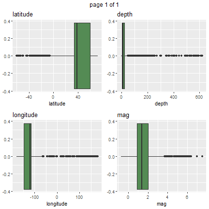
From above plots, it is put in evidence where most of such events are located and their magnitude and depth. The quantile function allows gathering more info about.
quantile(quakes$latitude, probs = c(0.1, 0.9), na.rm = TRUE)
##      10%      90%
## 19.15972 63.07784
quantile(quakes$longitude, probs = c(0.1, 0.9), na.rm = TRUE)
##        10%        90%
## -152.83000  -67.38542
quantile(quakes$depth, probs = c(0.1, 0.9), na.rm = TRUE)
##   10%   90%
##  0.97 59.00
quantile(quakes$mag, probs = c(0.1, 0.9), na.rm = TRUE)
##   10%   90%
## 0.470 3.216
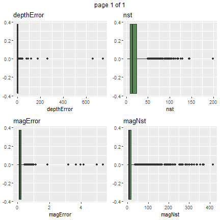
Box plots for remaining quantitative variables are shown.
grob_plots$chunk2

grob_plots$chunk3
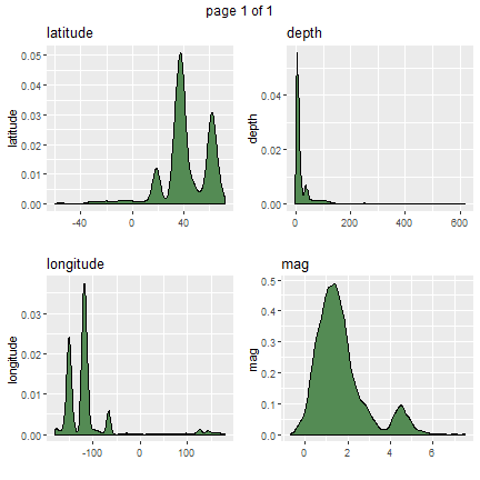
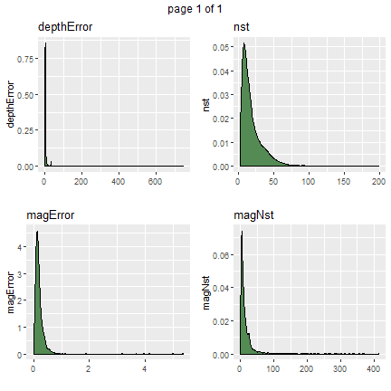
Density plots help to better visualize where most of the samples are. Using a similar routine where the geom_boxplot() is substituted with geom_density(), we show density plots for each quantitative variable.
gp <- invisible(lapply(quantitative_vars, function(x) {
  ggplot(data = quakes, aes(x=eval(parse(text=x)))) + geom_density(fill = "palegreen4") + ylab(x) + xlab("") + ggtitle(x) + theme(legend.position="none")}))
grob_plots <- invisible(lapply(chunk(1, length(gp), 4), function(x) {
  marrangeGrob(grobs=lapply(gp[x], ggplotGrob), nrow=2, ncol=2)}))
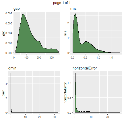
grob_plots$chunk1
grob_plots$chunk2
grob_plots$chunk3
We repeat the box plots by stratifying on event type (note the x=type within the plot aesthetic).
gp <- invisible(lapply(quantitative_vars, function(x) {
  ggplot(data = quakes, aes(x = type, y = eval(parse(text=x)))) + geom_boxplot(fill = "palegreen4") + ylab(x) + ggtitle(x) + theme(legend.position="none") + coord_flip()}))
grob_plots <- invisible(lapply(chunk(1, length(gp), 4), function(x) {
  marrangeGrob(grobs=lapply(gp[x], ggplotGrob), nrow=2, ncol=2)}))
grob_plots$chunk1
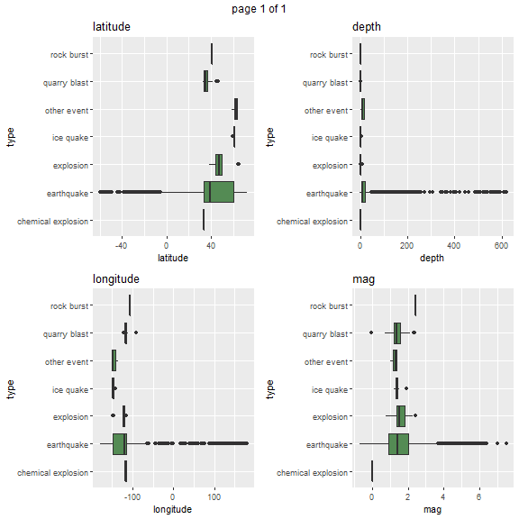
From above box plots, it is more evident the differentiation in values as dependent upon event types, especially for longitude and latitude.
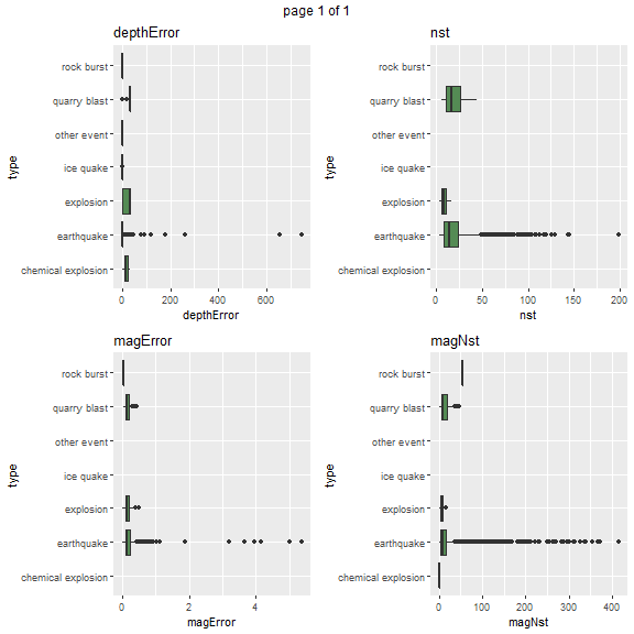
grob_plots$chunk2
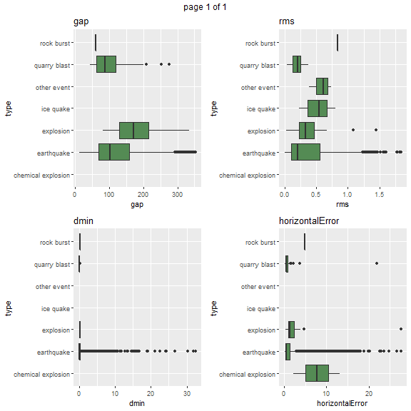
grob_plots$chunk3
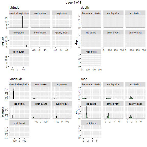
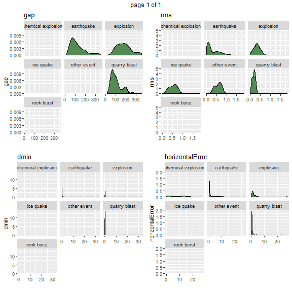
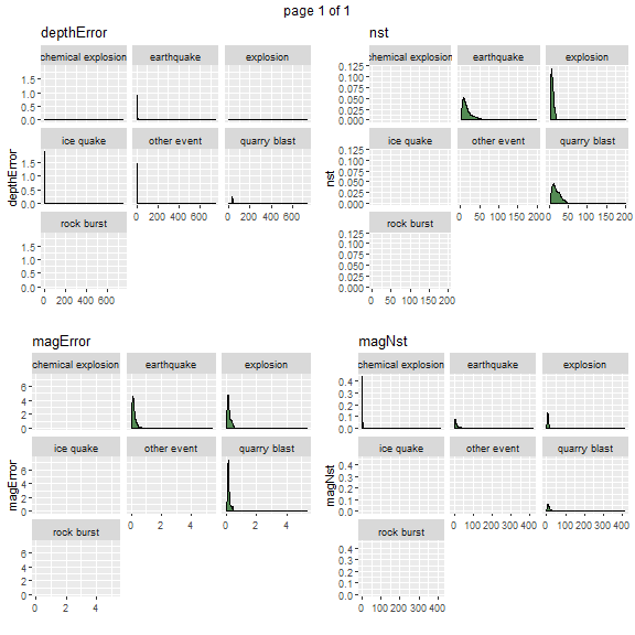
Density plots based on event type are shown.
gp <- invisible(lapply(quantitative_vars, function(x) {
  ggplot(data = quakes, aes(x=eval(parse(text=x)))) + geom_density(fill = "palegreen4") + ylab(x) + xlab("") + ggtitle(x) + theme(legend.position="none") + facet_wrap( ~ type)}))
grob_plots <- invisible(lapply(chunk(1, length(gp), 4), function(x) {
  marrangeGrob(grobs=lapply(gp[x], ggplotGrob), nrow=2, ncol=2)}))
grob_plots$chunk1
grob_plots$chunk2
grob_plots$chunk3
So far we investigated each quantitative variable by itself. In the prosecution of the analysis, we show graphics and tables highlighting the relationships among variables. The pair plots is one of the tool that can be used to infer relationships among pairs of variables. Further, we focus on the earthquake event type.
earthquakes <- quakes %>% filter(type == "earthquake")
pairs(earthquakes %>% select(quantitative_vars))
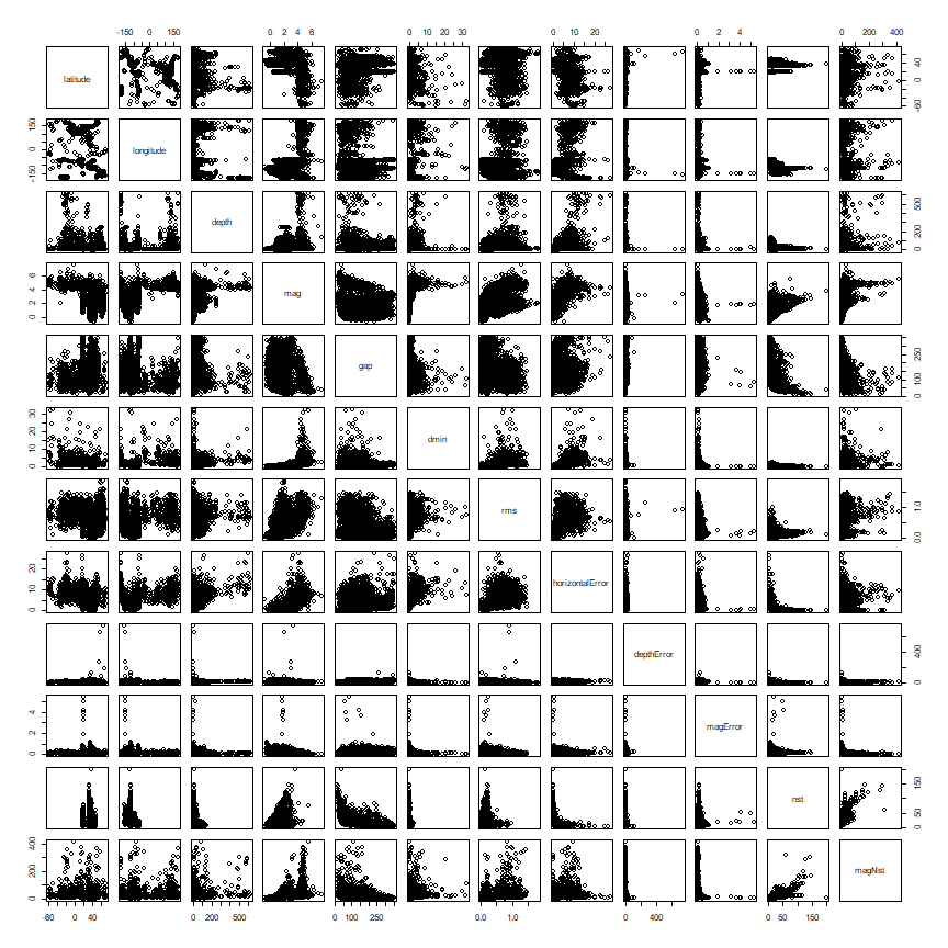
From the scatterplots above, we highlight one of the more interesting ones which shows earthquake magnitude against its depth.
hist_data <- earthquakes %>% select(mag, depth)
hist_data <- hist_data[complete.cases(hist_data),]

p <- ggplot(data = hist_data, aes(x = depth, y = mag)) + geom_point() + guides(fill=FALSE)
p
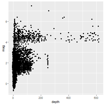
Above approximately 300 km, the registered magnitudes are greater than or equal 4 degrees. A third order relationship may be inferred (also a second order or a logarithmic may be attempted). Let us run a quick verification.
mag_depth_lr <- lm(mag ~ poly(depth, 3), data = hist_data)
summary(mag_depth_lr)
##
## Call:
## lm(formula = mag ~ poly(depth, 3), data = hist_data)
##
## Residuals:
##     Min      1Q  Median      3Q     Max
## -2.1845 -0.7333 -0.2310  0.4361  4.7112
##
## Coefficients:
##                  Estimate Std. Error t value Pr(>|t|)
## (Intercept)       1.65543    0.01177 140.625  < 2e-16 ***
## poly(depth, 3)1  40.93311    1.06794  38.329  < 2e-16 ***
## poly(depth, 3)2 -18.69337    1.06794 -17.504  < 2e-16 ***
## poly(depth, 3)3   6.64030    1.06794   6.218 5.29e-10 ***
## ---
## Signif. codes:  0 '***' 0.001 '**' 0.01 '*' 0.05 '.' 0.1 ' ' 1
##
## Residual standard error: 1.068 on 8226 degrees of freedom
## Multiple R-squared:  0.1807, Adjusted R-squared:  0.1804
## F-statistic: 604.7 on 3 and 8226 DF,  p-value: < 2.2e-16
All regressors are statistically significant. We then plot the original values against the fitted model.
p <- p + geom_point(aes(x = depth, y = fitted(mag_depth_lr)), colour = 'blue')
p

Correlation Analysis
Correlations are computed and collected as a table.
(cor_mat <- cor(quakes[, quantitative_vars], use = "pairwise.complete.obs"))
##                    latitude   longitude       depth         mag
## latitude         1.00000000 -0.52875417 -0.14867697 -0.38540388
## longitude       -0.52875417  1.00000000  0.14551789  0.55605921
## depth           -0.14867697  0.14551789  1.00000000  0.38277138
## mag             -0.38540388  0.55605921  0.38277138  1.00000000
## gap             -0.03794518  0.02975063  0.05196967  0.02808442
## dmin            -0.47773533  0.44108043  0.30279438  0.57339025
## rms              0.13784391  0.19709935  0.33147665  0.60872325
## horizontalError -0.53481018  0.61381314  0.54880413  0.76651963
## depthError      -0.06707420  0.06460787  0.03415940  0.08011669
## magError         0.02470576 -0.09122383 -0.06033724 -0.10270236
## nst             -0.11490376 -0.27741899 -0.04172062  0.28344750
## magNst          -0.19571866  0.26728165  0.26750233  0.46199100
##                         gap        dmin         rms horizontalError
## latitude        -0.03794518 -0.47773533  0.13784391     -0.53481018
## longitude        0.02975063  0.44108043  0.19709935      0.61381314
## depth            0.05196967  0.30279438  0.33147665      0.54880413
## mag              0.02808442  0.57339025  0.60872325      0.76651963
## gap              1.00000000  0.02719460  0.01882822      0.24321328
## dmin             0.02719460  1.00000000  0.53628845      0.65243264
## rms              0.01882822  0.53628845  1.00000000      0.75539036
## horizontalError  0.24321328  0.65243264  0.75539036      1.00000000
## depthError       0.32860091  0.08272005  0.03538935      0.26089694
## magError         0.10447472 -0.10511159 -0.12456313     -0.09591121
## nst             -0.49361171 -0.19298946  0.06461759     -0.24813050
## magNst          -0.18564633  0.28321115  0.42430650      0.29769313
##                  depthError    magError         nst      magNst
## latitude        -0.06707420  0.02470576 -0.11490376 -0.19571866
## longitude        0.06460787 -0.09122383 -0.27741899  0.26728165
## depth            0.03415940 -0.06033724 -0.04172062  0.26750233
## mag              0.08011669 -0.10270236  0.28344750  0.46199100
## gap              0.32860091  0.10447472 -0.49361171 -0.18564633
## dmin             0.08272005 -0.10511159 -0.19298946  0.28321115
## rms              0.03538935 -0.12456313  0.06461759  0.42430650
## horizontalError  0.26089694 -0.09591121 -0.24813050  0.29769313
## depthError       1.00000000 -0.01048942 -0.20439173 -0.01479938
## magError        -0.01048942  1.00000000 -0.07789094 -0.14474547
## nst             -0.20439173 -0.07789094  1.00000000  0.72021297
## magNst          -0.01479938 -0.14474547  0.72021297  1.00000000
The correlation plot allows for a more effective visualization of the same, with pie and number flavors.
corrplot(cor_mat, method = "pie", type = "lower", diag = FALSE)
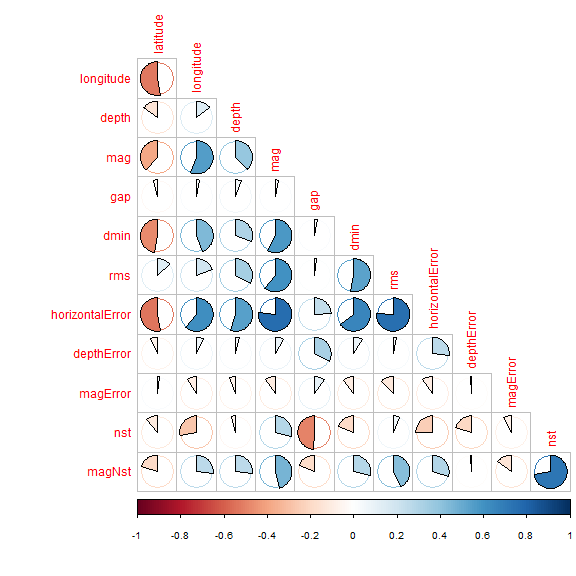
corrplot(cor_mat, method = "number", type = "lower", diag = FALSE)
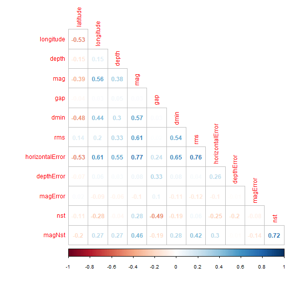
Strong correlations can be spotted for horizontal error against magnitude, dmin and rms. Further. between nst and magNst.
Maps
Having at our disposal longitude and latitude, it is worth showing a map of the earthquakes with color based upon their magnitude.
world <- map_data('world')

title <- paste("Earthquake map from ", paste(earthquakes$time[1], earthquakes$time[nrow(earthquakes)], sep = " to "))

p <- ggplot() + geom_map(data = world, map = world, aes(x = long, y=lat, group=group, map_id=region), fill="white", colour="#7f7f7f", size=0.5)
p <- p + geom_point(data = earthquakes, aes(x=longitude, y = latitude, colour = mag)) + scale_colour_gradient(low = "#00AA00",high = "#FF00AA") + ggtitle(title)
p
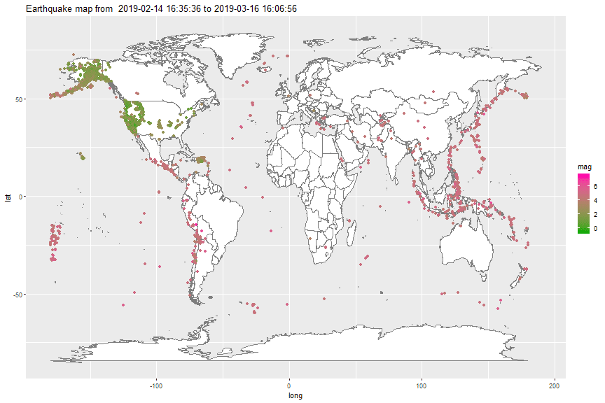
In the third post, we will go deeper in maps drawing. In the following post, we will analyze the categorical variables.
If you have any questions, please feel free to comment below.
References
- Earthquake dataset
- Eathquake dataset terms
- Introductory Statistics with R, 2nd Edition, P. Dalgaard, Springer
- Discrete Data Analysis with R, M. Friendly D. Meyer, CRC press