In this four-post series, I am going to analyze the Dow Jones Industrial Average (DJIA) index on years 2007-2018. The Dow Jones Industrial Average (DIJA) is a stock market index that indicates the value of thirty large, publicly owned companies based in the United States. The value of the DJIA is based upon the sum of the price of one share of stock for each component company. The sum is corrected by a factor which changes whenever one of the component stocks has a stock split or stock dividend. See ref. [1] for further details.
The main questions I will try to answer are:
- How the returns and trade volume have changed over the years?
- How the returns and trade volume volatility have changed over the years?
- How can we model the returns volatility?
- How can we model the trade volume volatility?
For the purpose, this post series is split as follows:
Part 1: getting data, summaries, and plots of daily and weekly log-returns
Part 2: getting data, summaries, and plots of daily trade volume and its log-ratio
Part 3: daily log-returns analysis and GARCH model definition
Part 4: daily trade volume analysis and GARCH model definition
Packages
The packages being used in this post series are herein listed.
suppressPackageStartupMessages(library(lubridate)) # dates manipulation
suppressPackageStartupMessages(library(fBasics)) # enhanced summary statistics
suppressPackageStartupMessages(library(lmtest)) # coefficients significance tests
suppressPackageStartupMessages(library(urca)) # unit rooit test
suppressPackageStartupMessages(library(ggplot2)) # visualization
suppressPackageStartupMessages(library(quantmod)) # getting financial data
suppressPackageStartupMessages(library(PerformanceAnalytics)) # calculating returns
suppressPackageStartupMessages(library(rugarch)) # GARCH modeling
suppressPackageStartupMessages(library(FinTS)) # ARCH test
suppressPackageStartupMessages(library(forecast)) # ARMA modeling
suppressPackageStartupMessages(library(strucchange)) # structural changes
suppressPackageStartupMessages(library(TSA)) # ARMA order identification
To the right, I added a short comment to highlight the main functionalities I took advantage from. Of course, those packages offer much more than just what I indicated.
Packages version are herein listed.
packages <- c("lubridate", "fBasics", "lmtest", "urca", "ggplot2", "quantmod", "PerformanceAnalytics", "rugarch", "FinTS", "forecast", "strucchange", "TSA")
version <- lapply(packages, packageVersion)
version_c <- do.call(c, version)
data.frame(packages=packages, version = as.character(version_c))
##                packages version
## 1             lubridate   1.7.4
## 2               fBasics 3042.89
## 3                lmtest  0.9.36
## 4                  urca   1.3.0
## 5               ggplot2   3.1.0
## 6              quantmod  0.4.13
## 7  PerformanceAnalytics   1.5.2
## 8               rugarch   1.4.0
## 9                 FinTS   0.4.5
## 10             forecast     8.4
## 11          strucchange   1.5.1
## 12                  TSA     1.2
The R language version running on Windows-10 is:
R.version
>##                _
## platform       x86_64-w64-mingw32
## arch           x86_64
## os             mingw32
## system         x86_64, mingw32
## status
## major          3
## minor          5.2
## year           2018
## month          12
## day            20
## svn rev        75870
## language       R
## version.string R version 3.5.2 (2018-12-20)
## nickname       Eggshell Igloo
Getting Data
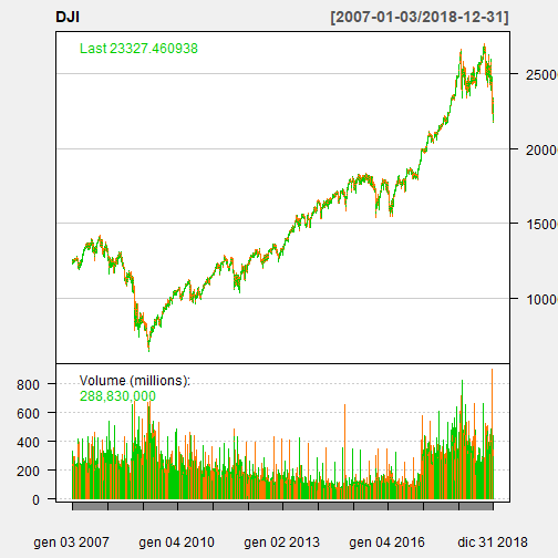
Taking advantage of the getSymbols() function made available within quantmod package we get Dow Jones Industrial Average from 2007 up to the end of 2018.
suppressMessages(getSymbols("^DJI", from = "2007-01-01", to = "2019-01-01"))
## [1] "DJI"
dim(DJI)
## [1] 3020    6
class(DJI)
## [1] "xts" "zoo"
Let us have a look at the DJI xts object which provides six-time series, as we can see.
head(DJI)
##            DJI.Open DJI.High  DJI.Low DJI.Close DJI.Volume DJI.Adjusted
## 2007-01-03 12459.54 12580.35 12404.82  12474.52  327200000     12474.52
## 2007-01-04 12473.16 12510.41 12403.86  12480.69  259060000     12480.69
## 2007-01-05 12480.05 12480.13 12365.41  12398.01  235220000     12398.01
## 2007-01-08 12392.01 12445.92 12337.37  12423.49  223500000     12423.49
## 2007-01-09 12424.77 12466.43 12369.17  12416.60  225190000     12416.60
## 2007-01-10 12417.00 12451.61 12355.63  12442.16  226570000     12442.16
tail(DJI)
##            DJI.Open DJI.High  DJI.Low DJI.Close DJI.Volume DJI.Adjusted
## 2018-12-21 22871.74 23254.59 22396.34  22445.37  900510000     22445.37
## 2018-12-24 22317.28 22339.87 21792.20  21792.20  308420000     21792.20
## 2018-12-26 21857.73 22878.92 21712.53  22878.45  433080000     22878.45
## 2018-12-27 22629.06 23138.89 22267.42  23138.82  407940000     23138.82
## 2018-12-28 23213.61 23381.88 22981.33  23062.40  336510000     23062.40
## 2018-12-31 23153.94 23333.18 23118.30  23327.46  288830000     23327.46
More precisely, we have available OHLC (Open, High, Low, Close) index value, adjusted close value and trade volume. Here we can see the corresponding chart as produced by the chartSeries within the quantmod package.
chartSeries(DJI, type = "bars", theme="white")
We herein analyse the adjusted close value.
dj_close <- DJI[,"DJI.Adjusted"]
Simple and log returns
Simple returns are defined as:
\[
R_{t}\ :=\ \frac{P_{t}}{P_{t-1}}\ \ -\ 1
\]
Log returns are defined as:
\[
r_{t}\ :=\ ln\frac{P_{t}}{P_{t-1}}\ =\ ln(1+R_{t})
\]
See ref. [4] for further details.
We compute log returns by taking advantage of CalculateReturns within PerformanceAnalytics package.
dj_ret <- CalculateReturns(dj_close, method = "log")
dj_ret <- na.omit(dj_ret)
Let us have a look.
head(dj_ret)
##             DJI.Adjusted
## 2007-01-04  0.0004945580
## 2007-01-05 -0.0066467273
## 2007-01-08  0.0020530973
## 2007-01-09 -0.0005547987
## 2007-01-10  0.0020564627
## 2007-01-11  0.0058356461
tail(dj_ret)
##            DJI.Adjusted
## 2018-12-21 -0.018286825
## 2018-12-24 -0.029532247
## 2018-12-26  0.048643314
## 2018-12-27  0.011316355
## 2018-12-28 -0.003308137
## 2018-12-31  0.011427645
This gives the following plot.
plot(dj_ret)
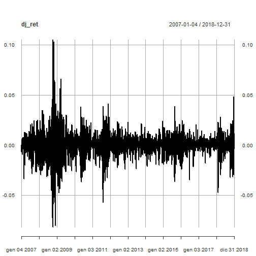
Sharp increases and decreases in volatility can be eye-balled. That will be in-depth verified in part 3.
Helper Functions
We need some helper functions to ease some basic data conversion, summaries and plots. Here below the details.
1. Conversion from xts to dataframe with year and value column. That allows for summarizations and plots on year basis.
xts_to_dataframe <- function(data_xts) {
  df_t <- data.frame(year = factor(year(index(data_xts))), value = coredata(data_xts))
  colnames(df_t) <- c( "year", "value")
  df_t
}
2. Enhanced summaries statistics for data stored as data frame columns.
bs_rn <- rownames(basicStats(rnorm(10,0,1))) # gathering the basic stats dataframe output row names that get lost with tapply()

dataframe_basicstats <- function(dataset) {
  result <- with(dataset, tapply(value, year, basicStats))
  df_result <- do.call(cbind, result)
  rownames(df_result) <- bs_rn
  as.data.frame(df_result)
}
3. Basic statistics dataframe row threshold filtering to return the associated column names.
filter_dj_stats <- function(dataset_basicstats, metricname, threshold) {
  r <- which(rownames(dataset_basicstats) ==  metricname)
  colnames(dataset_basicstats[r, which(dataset_basicstats[r,] > threshold), drop = FALSE])
}
4. Box-plots with faceting based on years.
dataframe_boxplot <- function(dataset, title) {
  p <- ggplot(data = dataset, aes(x = year, y = value)) + theme_bw() + theme(legend.position = "none") + geom_boxplot(fill = "lightblue")
  p <- p + theme(axis.text.x = element_text(angle = 90, hjust = 1)) + ggtitle(title) + ylab("year")
  p
}
5. Density plots with faceting based on years.
dataframe_densityplot <- function(dataset, title) {
  p <- ggplot(data = dataset, aes(x = value)) + geom_density(fill = "lightblue")
  p <- p + facet_wrap(. ~ year)
  p <- p + theme_bw() + theme(legend.position = "none") + ggtitle(title)
  p
}
6. QQ plots with faceting based on years.
dataframe_qqplot <- function(dataset, title) {
  p <- ggplot(data = dataset, aes(sample = value)) + stat_qq(colour = "blue") + stat_qq_line()
  p <- p + facet_wrap(. ~ year)
  p <- p + theme_bw() + theme(legend.position = "none") + ggtitle(title)
  p
}
7. Shapiro Test
shp_pvalue <- function (v) {
  shapiro.test(v)$p.value
}

dataframe_shapirotest <- function(dataset) {
 result <- with(dataset, tapply(value, year, shp_pvalue))
 as.data.frame(result)
}
Daily Log-returns Exploratory Analysis
We transform our original Dow Jones time series into a dataframe with year and value columns. That will ease plots and summaries by year.
dj_ret_df <- xts_to_dataframe(dj_ret)
head(dj_ret_df)
##   year         value
## 1 2007  0.0004945580
## 2 2007 -0.0066467273
## 3 2007  0.0020530973
## 4 2007 -0.0005547987
## 5 2007  0.0020564627
## 6 2007  0.0058356461
tail(dj_ret_df)
##      year        value
## 3014 2018 -0.018286825
## 3015 2018 -0.029532247
## 3016 2018  0.048643314
## 3017 2018  0.011316355
## 3018 2018 -0.003308137
## 3019 2018  0.011427645
Basic statistics summary
Basic statistics summary is given.
(dj_stats <- dataframe_basicstats(dj_ret_df))
##                   2007       2008       2009       2010       2011
## nobs        250.000000 253.000000 252.000000 252.000000 252.000000
## NAs           0.000000   0.000000   0.000000   0.000000   0.000000
## Minimum      -0.033488  -0.082005  -0.047286  -0.036700  -0.057061
## Maximum       0.025223   0.105083   0.066116   0.038247   0.041533
## 1. Quartile  -0.003802  -0.012993  -0.006897  -0.003853  -0.006193
## 3. Quartile   0.005230   0.007843   0.008248   0.004457   0.006531
## Mean          0.000246  -0.001633   0.000684   0.000415   0.000214
## Median        0.001098  -0.000890   0.001082   0.000681   0.000941
## Sum           0.061427  -0.413050   0.172434   0.104565   0.053810
## SE Mean       0.000582   0.001497   0.000960   0.000641   0.000837
## LCL Mean     -0.000900  -0.004580  -0.001207  -0.000848  -0.001434
## UCL Mean      0.001391   0.001315   0.002575   0.001678   0.001861
## Variance      0.000085   0.000567   0.000232   0.000104   0.000176
## Stdev         0.009197   0.023808   0.015242   0.010182   0.013283
## Skewness     -0.613828   0.224042   0.070840  -0.174816  -0.526083
## Kurtosis      1.525069   3.670796   2.074240   2.055407   2.453822
##                   2012       2013       2014       2015       2016
## nobs        250.000000 252.000000 252.000000 252.000000 252.000000
## NAs           0.000000   0.000000   0.000000   0.000000   0.000000
## Minimum      -0.023910  -0.023695  -0.020988  -0.036402  -0.034473
## Maximum       0.023376   0.023263   0.023982   0.038755   0.024384
## 1. Quartile  -0.003896  -0.002812  -0.002621  -0.005283  -0.002845
## 3. Quartile   0.004924   0.004750   0.004230   0.005801   0.004311
## Mean          0.000280   0.000933   0.000288  -0.000090   0.000500
## Median       -0.000122   0.001158   0.000728  -0.000211   0.000738
## Sum           0.070054   0.235068   0.072498  -0.022586   0.125884
## SE Mean       0.000470   0.000403   0.000432   0.000613   0.000501
## LCL Mean     -0.000645   0.000139  -0.000564  -0.001298  -0.000487
## UCL Mean      0.001206   0.001727   0.001139   0.001118   0.001486
## Variance      0.000055   0.000041   0.000047   0.000095   0.000063
## Stdev         0.007429   0.006399   0.006861   0.009738   0.007951
## Skewness      0.027235  -0.199407  -0.332766  -0.127788  -0.449311
## Kurtosis      0.842890   1.275821   1.073234   1.394268   2.079671
##                   2017       2018
## nobs        251.000000 251.000000
## NAs           0.000000   0.000000
## Minimum      -0.017930  -0.047143
## Maximum       0.014468   0.048643
## 1. Quartile  -0.001404  -0.005017
## 3. Quartile   0.003054   0.005895
## Mean          0.000892  -0.000231
## Median        0.000655   0.000695
## Sum           0.223790  -0.057950
## SE Mean       0.000263   0.000714
## LCL Mean      0.000373  -0.001637
## UCL Mean      0.001410   0.001175
## Variance      0.000017   0.000128
## Stdev         0.004172   0.011313
## Skewness     -0.189808  -0.522618
## Kurtosis      2.244076   2.802996
In the following, we make specific comments to some relevant aboveshown metrics.
Mean
Years when Dow Jones daily log-returns have positive mean values are:
filter_dj_stats(dj_stats, "Mean", 0)
## [1] "2007" "2009" "2010" "2011" "2012" "2013" "2014" "2016" "2017"
All Dow Jones daily log-returns mean values in ascending order.
dj_stats["Mean",order(dj_stats["Mean",,])]
##           2008      2018   2015     2011     2007    2012     2014
## Mean -0.001633 -0.000231 -9e-05 0.000214 0.000246 0.00028 0.000288
##          2010  2016     2009     2017     2013
## Mean 0.000415 5e-04 0.000684 0.000892 0.000933
Median
Years when Dow Jones daily log-returns have positive median are:
filter_dj_stats(dj_stats, "Median", 0)
## [1] "2007" "2009" "2010" "2011" "2013" "2014" "2016" "2017" "2018"
All Dow Jones daily log-returns median values in ascending order.
dj_stats["Median",order(dj_stats["Median",,])]
##            2008      2015      2012     2017     2010     2018     2014
## Median -0.00089 -0.000211 -0.000122 0.000655 0.000681 0.000695 0.000728
##            2016     2011     2009     2007     2013
## Median 0.000738 0.000941 0.001082 0.001098 0.001158
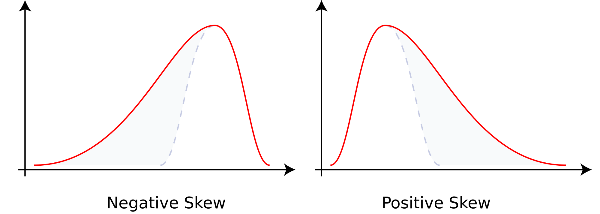
Skewness
A spatial distribution has positive skewness when it has tendency to produce more positive extreme values above rather than negative ones. Negative skew commonly indicates that the tail is on the left side of the distribution, and positive skew indicates that the tail is on the right. Here is a sample picture to explain.
Years when Dow Jones daily log-returns have positive skewness are:
filter_dj_stats(dj_stats, "Skewness", 0)
## [1] "2008" "2009" "2012"
All Dow Jones daily log-returns skewness values in ascending order.
dj_stats["Skewness",order(dj_stats["Skewness",,])]
##               2007      2011      2018      2016      2014      2013
## Skewness -0.613828 -0.526083 -0.522618 -0.449311 -0.332766 -0.199407
##               2017      2010      2015     2012    2009     2008
## Skewness -0.189808 -0.174816 -0.127788 0.027235 0.07084 0.224042
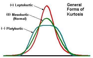
Excess Kurtosis
The Kurtosis is a measure of the “tailedness” of the probability distribution of a real-valued random variable. The kurtosis of any univariate normal distribution is 3. The excess kurtosis is equal to the kurtosis minus 3 and eases the comparison to the normal distribution. The basicStats function within the fBasics package reports the excess kurtosis. Here is a sample picture to explain.
Years when Dow Jones daily log-returns have positive excess kurtosis are:
filter_dj_stats(dj_stats, "Kurtosis", 0)
##  [1] "2007" "2008" "2009" "2010" "2011" "2012" "2013" "2014" "2015" "2016"
## [11] "2017" "2018"
All Dow Jones daily log-returns excess kurtosis values in ascending order.
dj_stats["Kurtosis",order(dj_stats["Kurtosis",,])]
##             2012     2014     2013     2015     2007     2010    2009
## Kurtosis 0.84289 1.073234 1.275821 1.394268 1.525069 2.055407 2.07424
##              2016     2017     2011     2018     2008
## Kurtosis 2.079671 2.244076 2.453822 2.802996 3.670796
Year 2018 has the closest excess kurtosis to 2008.
Box-plots
dataframe_boxplot(dj_ret_df, "DJIA daily log-returns box plots 2007-2018")
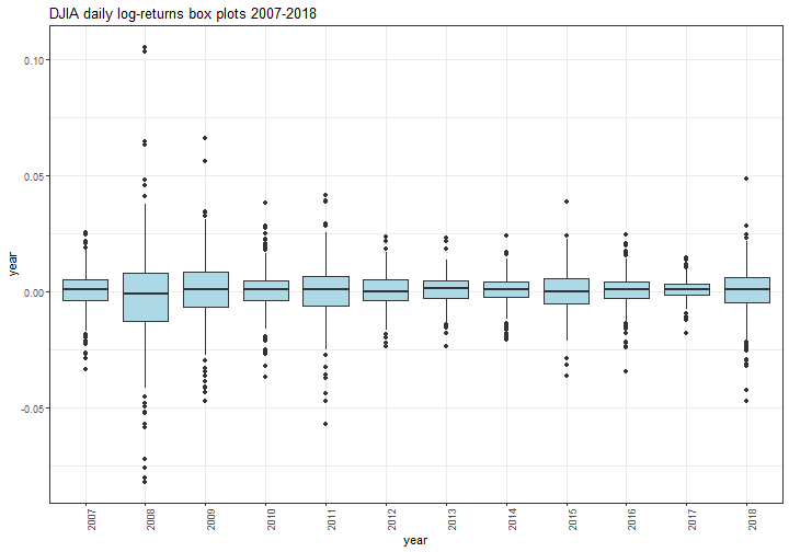
We can see how the most extreme values occurred on 2008. Starting on 2009, the values range gets narrow, with the exception of 2011 and 2015. However, comparing 2017 with 2018, it is remarkable an improved tendency to produce more extreme values on last year.
Density plots
dataframe_densityplot(dj_ret_df, "DJIA daily log-returns density plots 2007-2018")
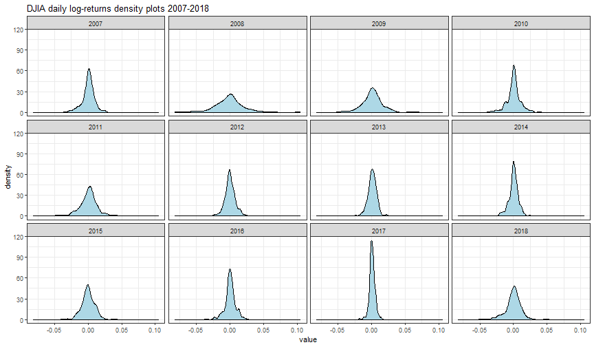
Year 2007 has remarkable negative skewness. Year 2008 is characterized by flatness and extreme values. The 2017 peakness is in constrant with the flatness and left skeweness of 2018 results.
Shapiro Tests
dataframe_shapirotest(dj_ret_df)
##            result
## 2007 5.989576e-07
## 2008 5.782666e-09
## 2009 1.827967e-05
## 2010 3.897345e-07
## 2011 5.494349e-07
## 2012 1.790685e-02
## 2013 8.102500e-03
## 2014 1.750036e-04
## 2015 5.531137e-03
## 2016 1.511435e-06
## 2017 3.304529e-05
## 2018 1.216327e-07
The null hypothesis of normality is rejected for all years 2007-2018.
QQ plots
dataframe_qqplot(dj_ret_df, "DJIA daily log-returns QQ plots 2007-2018")
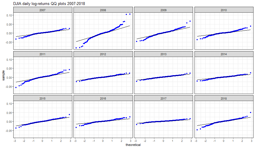
Strong departure from normality of daily log returns (and hence log-normality for discrete returns) is visible on years 2008, 2009, 2010, 2011 and 2018.
Weekly Log-returns Exploratory Analysis
The weekly log returns can be computed starting from the daily ones. Let us suppose to analyse the trading week on days {t-4, t-3, t-2, t-1, t} and to know closing price at day t-5 (last day of the previous week). We define the weekly log-return as:
\[
r_{t}^{w}\ :=\ ln \frac{P_{t}}{P_{t-5}}
\]
That can be rewritten as:
\[
\begin{equation}
\begin{aligned}
r_{t}^{w}\ = \ ln \frac{P_{t}P_{t-1} P_{t-2} P_{t-3} P_{t-4}}{P_{t-1} P_{t-2} P_{t-3} P_{t-4} P_{t-5}} = \\
=\ ln \frac{P_{t}}{P_{t-1}} + ln \frac{P_{t-1}}{P_{t-2}} + ln \frac{P_{t-2}}{P_{t-3}} + ln \frac{P_{t-3}}{P_{t-4}}\ +\ ln \frac{P_{t-4}}{P_{t-5}}\ = \\ =
r_{t} + r_{t-1} + r_{t-2} + r_{t-3} + r_{t-4}
\end{aligned}
\end{equation}
\]
Hence the weekly log return is the sum of daily log returns applied to the trading week window.
We take a look at Dow Jones weekly log-returns.
dj_weekly_ret <- apply.weekly(dj_ret, sum)
plot(dj_weekly_ret)
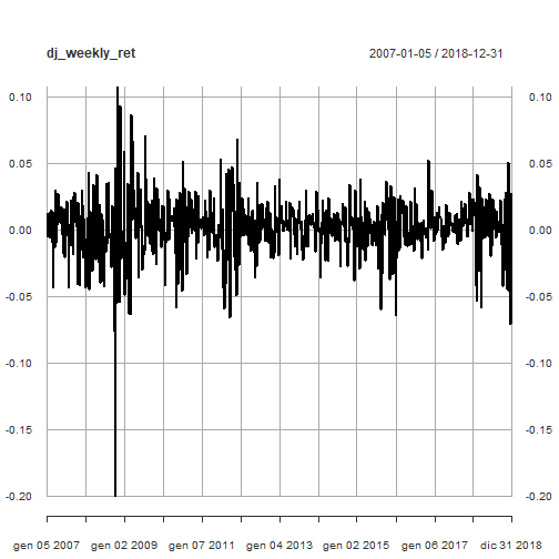
That plot shows sharp increses and decreases of volatility.
We transform the original time series data and index into a dataframe.
dj_weekly_ret_df <- xts_to_dataframe(dj_weekly_ret)
dim(dj_weekly_ret_df)
## [1] 627   2
head(dj_weekly_ret_df)
##   year         value
## 1 2007 -0.0061521694
## 2 2007  0.0126690596
## 3 2007  0.0007523559
## 4 2007 -0.0062677053
## 5 2007  0.0132434177
## 6 2007 -0.0057588519
tail(dj_weekly_ret_df)
##     year       value
## 622 2018  0.05028763
## 623 2018 -0.04605546
## 624 2018 -0.01189714
## 625 2018 -0.07114867
## 626 2018  0.02711928
## 627 2018  0.01142764
Basic statistics summary
(dj_stats <- dataframe_basicstats(dj_weekly_ret_df))
##                  2007      2008      2009      2010      2011      2012
## nobs        52.000000 52.000000 53.000000 52.000000 52.000000 52.000000
## NAs          0.000000  0.000000  0.000000  0.000000  0.000000  0.000000
## Minimum     -0.043199 -0.200298 -0.063736 -0.058755 -0.066235 -0.035829
## Maximum      0.030143  0.106977  0.086263  0.051463  0.067788  0.035316
## 1. Quartile -0.009638 -0.031765 -0.015911 -0.007761 -0.015485 -0.010096
## 3. Quartile  0.014808  0.012682  0.022115  0.016971  0.014309  0.011887
## Mean         0.001327 -0.008669  0.003823  0.002011  0.001035  0.001102
## Median       0.004244 -0.006811  0.004633  0.004529  0.001757  0.001166
## Sum          0.069016 -0.450811  0.202605  0.104565  0.053810  0.057303
## SE Mean      0.002613  0.006164  0.004454  0.003031  0.003836  0.002133
## LCL Mean    -0.003919 -0.021043 -0.005115 -0.004074 -0.006666 -0.003181
## UCL Mean     0.006573  0.003704  0.012760  0.008096  0.008736  0.005384
## Variance     0.000355  0.001975  0.001051  0.000478  0.000765  0.000237
## Stdev        0.018843  0.044446  0.032424  0.021856  0.027662  0.015382
## Skewness    -0.680573 -0.985740  0.121331 -0.601407 -0.076579 -0.027302
## Kurtosis    -0.085887  5.446623 -0.033398  0.357708  0.052429 -0.461228
##                  2013      2014      2015      2016      2017      2018
## nobs        52.000000 52.000000 53.000000 52.000000 52.000000 53.000000
## NAs          0.000000  0.000000  0.000000  0.000000  0.000000  0.000000
## Minimum     -0.022556 -0.038482 -0.059991 -0.063897 -0.015317 -0.071149
## Maximum      0.037702  0.034224  0.037693  0.052243  0.028192  0.050288
## 1. Quartile -0.001738 -0.006378 -0.012141 -0.007746 -0.002251 -0.011897
## 3. Quartile  0.011432  0.010244  0.009620  0.012791  0.009891  0.019857
## Mean         0.004651  0.001756 -0.000669  0.002421  0.004304 -0.001093
## Median       0.006360  0.003961  0.000954  0.001947  0.004080  0.001546
## Sum          0.241874  0.091300 -0.035444  0.125884  0.223790 -0.057950
## SE Mean      0.001828  0.002151  0.002609  0.002436  0.001232  0.003592
## LCL Mean     0.000981 -0.002563 -0.005904 -0.002470  0.001830 -0.008302
## UCL Mean     0.008322  0.006075  0.004567  0.007312  0.006778  0.006115
## Variance     0.000174  0.000241  0.000361  0.000309  0.000079  0.000684
## Stdev        0.013185  0.015514  0.018995  0.017568  0.008886  0.026154
## Skewness    -0.035175 -0.534403 -0.494963 -0.467158  0.266281 -0.658951
## Kurtosis    -0.200282  0.282354  0.665460  2.908942 -0.124341 -0.000870
In the following, we make specific comments to some relevant aboveshown metrics.
Mean
Years when Dow Jones weekly log-returns have positive mean are:
filter_dj_stats(dj_stats, "Mean", 0)
## [1] "2007" "2009" "2010" "2011" "2012" "2013" "2014" "2016" "2017"
All mean values in ascending order.
dj_stats["Mean",order(dj_stats["Mean",,])]
##           2008      2018      2015     2011     2012     2007     2014
## Mean -0.008669 -0.001093 -0.000669 0.001035 0.001102 0.001327 0.001756
##          2010     2016     2009     2017     2013
## Mean 0.002011 0.002421 0.003823 0.004304 0.004651
Median
Years when Dow Jones weekly log-returns have positive median are:
filter_dj_stats(dj_stats, "Median", 0)
##  [1] "2007" "2009" "2010" "2011" "2012" "2013" "2014" "2015" "2016" "2017"
## [11] "2018"
All median values in ascending order.
dj_stats["Median",order(dj_stats["Median",,])]
##             2008     2015     2012     2018     2011     2016     2014
## Median -0.006811 0.000954 0.001166 0.001546 0.001757 0.001947 0.003961
##           2017     2007     2010     2009    2013
## Median 0.00408 0.004244 0.004529 0.004633 0.00636
Skewness
Years when Dow Jones weekly log-returns have positive skewness are:
filter_dj_stats(dj_stats, "Skewness", 0)
## [1] "2009" "2017"
All skewness values in ascending order.
dj_stats["Skewness",order(dj_stats["Skewness",,])]
##              2008      2007      2018      2010      2014      2015
## Skewness -0.98574 -0.680573 -0.658951 -0.601407 -0.534403 -0.494963
##               2016      2011      2013      2012     2009     2017
## Skewness -0.467158 -0.076579 -0.035175 -0.027302 0.121331 0.266281
Excess Kurtosis
Years when Dow Jones weekly log-returns have positive excess kurtosis are:
filter_dj_stats(dj_stats, "Kurtosis", 0)
## [1] "2008" "2010" "2011" "2014" "2015" "2016"
All excess kurtosis values in ascending order.
dj_stats["Kurtosis",order(dj_stats["Kurtosis",,])]
##               2012      2013      2017      2007      2009     2018
## Kurtosis -0.461228 -0.200282 -0.124341 -0.085887 -0.033398 -0.00087
##              2011     2014     2010    2015     2016     2008
## Kurtosis 0.052429 0.282354 0.357708 0.66546 2.908942 5.446623
Year 2008 has also highest weekly kurtosis. However in this scenario, 2017 has negative kurtosis and year 2016 has the second highest kurtosis.
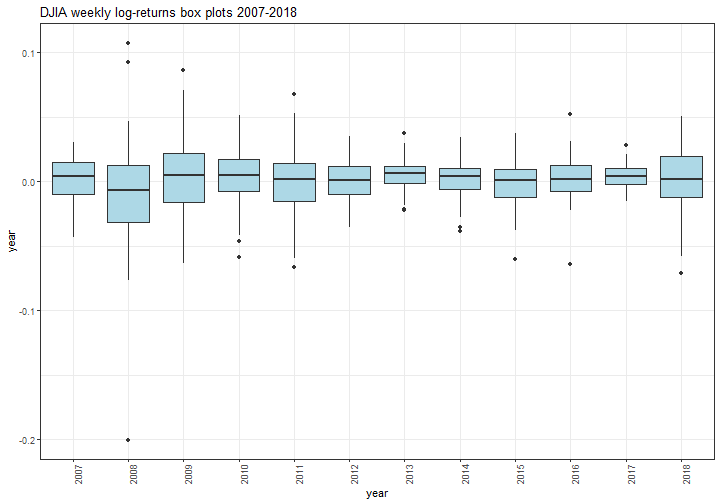
Box-plots
dataframe_boxplot(dj_weekly_ret_df, "DJIA weekly log-returns box plots 2007-2018")
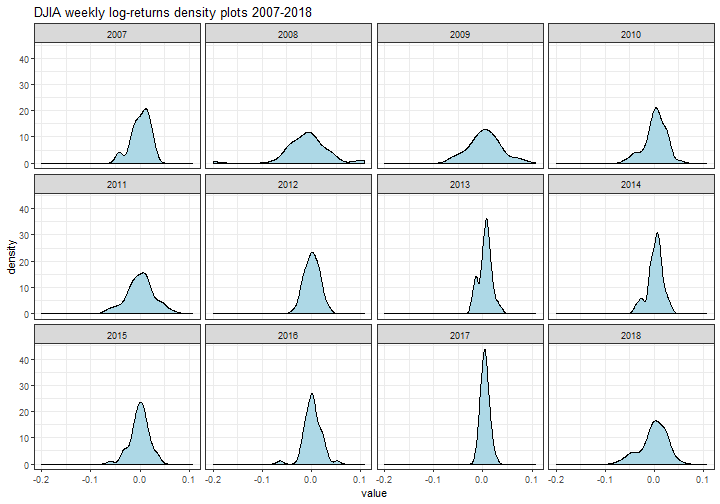
Density plots
dataframe_densityplot(dj_weekly_ret_df, "DJIA weekly log-returns density plots 2007-2018")
Shapiro Tests
dataframe_shapirotest(dj_weekly_ret_df)
##            result
## 2007 0.0140590311
## 2008 0.0001397267
## 2009 0.8701335006
## 2010 0.0927104389
## 2011 0.8650874270
## 2012 0.9934600084
## 2013 0.4849043121
## 2014 0.1123139646
## 2015 0.3141519756
## 2016 0.0115380989
## 2017 0.9465281164
## 2018 0.0475141869
The null hypothesis of normality is rejected for years 2007, 2008, 2016.
QQ plots
dataframe_qqplot(dj_weekly_ret_df, "DJIA weekly log-returns QQ plots 2007-2018")
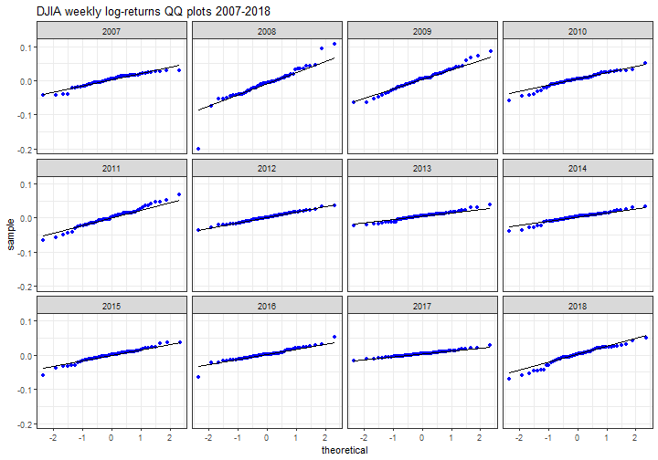
Strong departure from normality is particularly visible on year 2008.
Saving the current enviroment for further analysis.
save.image(file='DowEnvironment.RData')
If you have any questions, please feel free to comment below.
References
- Dow Jones Industrial Average
- Skewness
- Kurtosis
- An introduction to analysis of financial data with R, Wiley, Ruey S. Tsay
- Time series analysis and its applications, Springer ed., R.H. Shumway, D.S. Stoffer
- Applied Econometric Time Series, Wiley, W. Enders, 4th ed.]
- Forecasting – Principle and Practice, Texts, R.J. Hyndman
- Options, Futures and other Derivatives, Pearson ed., J.C. Hull
- An introduction to rugarch package
- Applied Econometrics with R, Achim Zeileis, Christian Kleiber – Springer Ed.
- GARCH modeling: diagnostic tests
Disclaimer
Any securities or databases referred in this post are solely for illustration purposes, and under no regard should the findings presented here be interpreted as investment advice or promotion of any particular security or source.