Find the best predictive model using R/caret package/modelgrid

It's tough to make predictions, especially about the future (Yogi Berra), but I think the way to get there shouldn't be.

I have built a new shiny application BMuCaret to fit and evaluate multiple classifiers and select the best one, which achieves the best performance for a given data **. The area under the ROC curve (not the curve) has been considered as a key metric to measure the model performance.

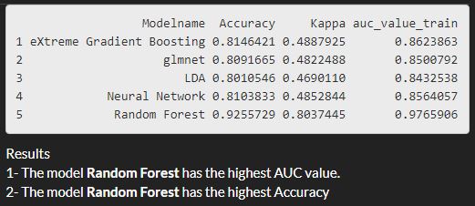
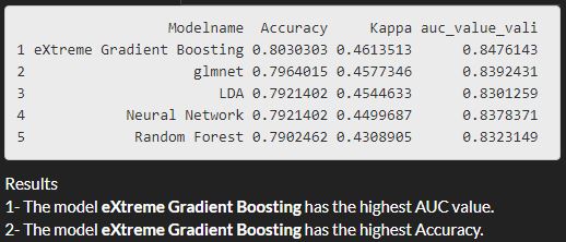
With this new application (BMuCaret: Best Model using Caret) I evaluate five classifiers arising from 5 families (discriminant analysis, neural networks, support vector machines, Generalized Linear Models, random forests) and identify the classifier with the highest AUC. On the training data the Random Forest classifier(method: rf) tends to perform well **but on the validation data, the eXtreme Gradient Boosting classifier(method: xgbDART) is performing better and gives better results in respect to the AUC and to the model accuracy as well.

The AUC/Accuracy/Kappa on the training set:

The AUC/Accuracy/Kappa on the validation set:

Concept

In order to perform a fair comparison of the candidate classifiers:

1. I will use the same training/test split.
2. The learning problem(as an example) is the binary classification problem; predict customer churn. the data set can be found here.
3. Data pre-Processing has been performed using the recipe method.
4. A common setting/trainControl will be created, which will be shared by all considered classifiers(this will allow us to fit the models under the same conditions).
5. For tuning the hyperparameters the method adaptive_cv will be used (also allow us to reduce the tuning time).

I use the following candidate classifiers:

• eXtreme Gradient Boosting (method: xgbDART).
• glmnet (method glmnet).
• Linear discriminant analysis (method: lda).
• Neural Network (method: nnet).
• Random Forest (method : rf).

This list can be expanded with further classifiers by using the add_model function from the model grid package.

The caret and modelgrid packages are used to train and to evaluate the candidate models ( For a very accessible introduction to caret and modelgid please have a look at here and here).
DataExplorer packet has been used to explore the data.

Here is the code

Data set preprocessing (Module1)
It will return a clean data set, and the partition of the data set into training and validation data set.

library(shiny)

library(shinythemes)
library(modelgrid)
library(magrittr)
library(caret)
library(foreach)
library(recipes)

library(plyr)
library(purrr)
library(dplyr)
library(pROC)
library(BradleyTerry2)
library(corrplot)
library(DataExplorer)
library(randomForest)
library(glmnet)
library(xgboost)
library(e1071)

#######################################
# load data
set.seed(9650)
Telco_custumer_2 <- read.csv("Telco_customer_2.csv")
data_set <- Telco_custumer_2
data_set <- data_set%>%dplyr::select(-"customerID") 
data_set$Churn <- as.factor(data_set$Churn)
######################################
# Pre-Processing the data Telco_Customer_Churn  using recipe
set.seed(9650)
Attri_rec_2 <- 
    recipe(Churn ~ ., data = data_set) %>%        # Formula.
    step_dummy(all_predictors())%>%               # convert nominal data into one or more numeric.
    step_knnimpute(all_predictors())%>%           # impute missing data using nearest neighbors.
    step_zv(all_predictors()) %>%                 # remove variables that are highly sparse and unbalanced.
    step_corr(all_predictors()) %>%               # remove variables that have large absolute correlations with 
                                                  # other variables.
    step_center(all_predictors()) %>%             # normalize numeric data to have a mean of zero.
    step_scale(all_predictors()) %>%              # normalize numeric data to have a standard deviation of one.
    prep(training = data_set, retain = TRUE)      # train the data recipe 


## Warning: The following variables are not factor vectors and will be
## ignored: `SeniorCitizen`, `tenure`, `MonthlyCharges`, `TotalCharges`

data_rec_2 <- as.data.frame(juice(Attri_rec_2))
# add the response variable
data_rec_2$Churn <- data_set$Churn
# str(data_rec_2)
# Create a Validation Dataset (training data 70% and validation data 30% of the original data)
set.seed(9650)
validation_index <- createDataPartition(data_rec_2$Churn,times= 1,  p= 0.70, list=FALSE)
# select 30% of the data for validation
data_validation <- data_rec_2[-validation_index,]
# use the remaining 70% of data to train the models
data_train <- data_rec_2[validation_index, ]
# For traing the models  
x_train <- data_train%>%select(-Churn) # Predictors
y_train <- data_train[["Churn"]] # Response
# for validation/test
x_validation <- data_validation%>%select(-Churn)
y_validation <- data_validation[["Churn"]]

Construct model grid and define shared settings (Module2)

set.seed(9650)
mg <- 
    model_grid() %>%
    share_settings(
        y = y_train,
        x = x_train,
        metric = "ROC",
        trControl = trainControl(
            method = "adaptive_cv",
            number = 10, repeats = 5,
            adaptive = list(min =3, alpha =0.05, method = "BT", complete = FALSE),
            search = "random",
            summaryFunction = twoClassSummary,
            classProbs = TRUE))
purrr::map_chr(mg$shared_settings, class)

##            y            x       metric    trControl 
##     "factor" "data.frame"  "character"       "list"

# add models to train
mg_final <- mg %>%
    add_model(model_name = "LDA",
              method = "lda",
              custom_control = list(method = "repeatedcv",
                                    number = 10,
                                    repeats =5))%>%
    add_model(model_name = "eXtreme Gradient Boosting",
              method = "xgbDART") %>%
    add_model(model_name = "Neural Network", 
              method = "nnet")%>%
    add_model(model_name = "glmnet",
              method = "glmnet")%>%
    add_model(model_name = "Random Forest", 
              method = "rf")
    # %>% add_model(model_name = "gbm",
              # method="gbm",
              # custom_control = list(verbose = FALSE))
list_model <- c(names(mg_final$models))

The code for the BMuCaret Shiny application (Module3)

################################# Define UI #########################
ui <- fluidPage(theme = shinytheme("slate"),
# Application title
  titlePanel(wellPanel("Find the best predictive model using R/caret package/modelgrid",br(),"BMuCaret")),
    navbarPage("Workflow ===>",
      tabPanel("Exploratory Data Analysis",
        tabsetPanel(type = "tabs",
          tabPanel("Explore the data object",
            navlistPanel(
              tabPanel("1- Structure of the data object", verbatimTextOutput("str_ucture")),
                tabPanel("2- Missing values ?", plotOutput("missing_value")),
                tabPanel("3- Correlation analysis", plotOutput("coor_plot", height = 700)))),

          tabPanel("After Data Cleaning (using recipe method)",
            navlistPanel(
              tabPanel("1- Structure of the data object after Processing", verbatimTextOutput("str_ucture_after")),
                tabPanel("2- Missing values ?", plotOutput("missing_value_after") ),
                tabPanel("3- Correlation analysis after", plotOutput("coor_plot_after", height = 600))
                                  )))),
          tabPanel("Fitting & Validation & Statistics",
            sidebarLayout(
              sidebarPanel(
                wellPanel(selectInput(inputId = "abd", 
                                      label = "Model choose : ",
                                      choices = c("none", list_model),
                                      selected = "none"))),
        mainPanel(
          tabsetPanel(type= "tabs",
            tabPanel("Model Training & Summary",
              navlistPanel(
                tabPanel("1- Show info model grid ",verbatimTextOutput("info_modelgrid")),
                tabPanel("2- Performance statistics of the model grid (dotplot) ", 
                                plotOutput("dotplot", width = 600, height = 600)),
                tabPanel("3- Extract Performance of the model grid ", 
                                verbatimTextOutput(outputId = "summary")),
                tabPanel("4- Show the AUC & Accuracy of individual models (on data training)", 
                                verbatimTextOutput("Accurac_AUC"), htmlOutput("best_model_train")),
                tabPanel("5- Show Statistics of individual model", 
                                verbatimTextOutput(outputId = "Indiv_Analysis")
                                ,"Examine the relationship between the estimates of performance 
                                and the tuning parameters", br(),
                                plotOutput(outputId= "tuning_parameter")),
                tabPanel("6- Show single model's Accuracy (on data training)",
                                verbatimTextOutput(outputId = "accuracy")))),
# output model validation and statistics      
            tabPanel("Model Validation & Statistics", 
              navlistPanel(
                tabPanel("1-Show the AUC & Accuracy of individual models (on validation data)", 
                              verbatimTextOutput(outputId = "AUC_of_individ"), 
                              htmlOutput("best_model_vali")),
                tabPanel("2- Show single model's Accuracy/data validation", 
                              verbatimTextOutput("accuracy_vali")),
                tabPanel("3- Plot variable importance", plotOutput("variable_imp"))))
  )))),
              tabPanel("Next: Model Interpretation")
),

br(), br(),br(), 

h5("BMuCaret App. built with", img(src = "https://www.rstudio.com/wp-content/uploads/2014/04/shiny-200x232.png", 
                                     height= "30px"), 
   "by",
br(), 
"Author: Abderrahim Lyoubi-Idrissi", 
br(),
"Contact: [email protected]")
)
################################# Define server logic #########################
server <- function(input, output) {
set.seed(9650)    
# before processing the data
# data structure
    output$str_ucture <- renderPrint({
        str(data_set)
    })
# Missing values ? 
    output$missing_value <- renderPlot({
        plot_missing(data_set)
    })
# plot to check the results of step_corr(all_predictors())
    output$coor_plot <- renderPlot({
        plot_correlation(data_set)
    })
## after processing the data 
# data structure
    output$str_ucture_after <- renderPrint({
        str(data_rec_2)
    })
# plot to check the missing values
    output$missing_value_after <- renderPlot({
        plot_missing(data_rec_2)
    })
 # plot to check the correlation
    output$coor_plot_after <- renderPlot({
        plot_correlation(data_rec_2)
    })
set.seed(9650)
# Infos about the componets of the constructed model grid     
    output$info_modelgrid <- renderPrint({
        mg_final$models
    })
# train all models 
    set.seed(9650)
    mg_final_tra <- reactive({train(mg_final)})
    ## plot to compare
    output$dotplot <- renderPlot({ 
        mg_final_tra()$model_fits %>%
            caret::resamples(.) %>%
            lattice::dotplot(.)
    })
# Show the overall summary
    set.seed(9650)
    output$summary <- renderPrint({
        mg_final_tra()$model_fits %>%
            caret::resamples(.) %>%
            summary(.)
    })
# computing the auc & the accuracy (on train data)
    set.seed(9650)
    output$Accurac_AUC <- renderPrint({
    AUC1 <- mg_final_tra()$model_fits%>% predict(., newdata = x_train, type ="prob")%>%map(~roc(y_train, .x[,2]))
    auc_value_train <- map_dbl(AUC1, ~(.x)$auc)
    auc_value_df_train_df <- as.data.frame(auc_value_train)
    accuarcy_all_train <- predict(mg_final_tra()$model_fits, newdata = x_train)%>% 
        map( ~confusionMatrix(.x, y_train))%>%
        map_dfr(~ cbind(as.data.frame(t(.x$overall)),as.data.frame(t(.x$byClass))), .id = "Modelname")%>%
        select(Modelname, Accuracy, Kappa)
    accuracy_auc_train <-  bind_cols(accuarcy_all_train,auc_value_df_train_df)
    print(accuracy_auc_train)
    })
# computing the auc and the Accuracy
    set.seed(9650)
    output$best_model_train <- renderUI({
    AUC1 <- mg_final_tra()$model_fits%>% predict(., newdata = x_train, type ="prob")%>%
        map(~roc(y_train, .x[,2])) 
    auc_value_train <- map_dbl(AUC1, ~(.x)$auc)
    auc_value_df_train_df <- as.data.frame(auc_value_train)
    accuarcy_all_train <- predict(mg_final_tra()$model_fits, newdata = x_train)%>% 
        map( ~confusionMatrix(.x, y_train))%>%
        map_dfr(~ cbind(as.data.frame(t(.x$overall)),as.data.frame(t(.x$byClass))), .id = "Modelname")%>%
        select(Modelname, Accuracy, Kappa)
    accuracy_auc_train <-  bind_cols(accuarcy_all_train, auc_value_df_train_df)
    max_auc_train <- filter(accuracy_auc_train, auc_value_train == max(accuracy_auc_train$auc_value_train))%>%
                    select(Modelname)
    max_Accuracy_train <- filter(accuracy_auc_train, Accuracy == max(accuracy_auc_train$Accuracy))%>%
                    select(Modelname)

    HTML(paste("Results", br(),  
                   "1- The model", strong(max_auc_train), "has the highest AUC value.", br(),
                   "2- The model",strong(max_Accuracy_train), "has the highest Accuracy" ))
    })
# Show the summary of individual model    
    output$Indiv_Analysis <- renderPrint({if(input$abd == "none"){print("Please select a model")}
                mg_final_tra()$model_fits[[input$abd]]
    })
# Plot the individual model    
    output$tuning_parameter <- renderPlot({
        ggplot( mg_final_tra()$model_fits[[input$abd]])
    })
# ConfusionMatrix on training data        
    output$accuracy <- renderPrint({if(input$abd == "none"){print("Please select a model")}
        else{
        confusionMatrix( predict(mg_final_tra()$model_fits[[input$abd]], x_train), y_train)}
    })
################################### Validation #########################
# Extract the auc values
    output$AUC_of_individ <- renderPrint({
      AUC2 <- mg_final_tra()$model_fits%>% predict(., newdata = x_validation, type ="prob")%>% 
            map(~roc(y_validation, .x[,2]))
      auc_value_vali <- map_dbl(AUC2, ~(.x)$auc)
      auc_value_df_vali_df <- as.data.frame(auc_value_vali)
      cf_vali <- predict(mg_final_tra()$model_fits, newdata = x_validation)%>% 
                            map( ~confusionMatrix(.x, y_validation))
      cf_vali%>%
        map_dfr(~ cbind(as.data.frame(t(.x$overall)),as.data.frame(t(.x$byClass))), .id = "Modelname")%>% 
                            select(Modelname, Accuracy, Kappa)
      accuarcy_all_vali <- predict(mg_final_tra()$model_fits, newdata = x_validation)%>% 
                            map( ~confusionMatrix(.x, y_validation))%>%
                            map_dfr(~ cbind(as.data.frame(t(.x$overall)),
                                      as.data.frame(t(.x$byClass))), .id = "Modelname")%>%
                                      select(Modelname, Accuracy, Kappa)
      accuracy_auc_vali <-  bind_cols(accuarcy_all_vali,auc_value_df_vali_df) 
      print(accuracy_auc_vali)
    })
    output$best_model_vali <- renderUI({
      AUC2 <- mg_final_tra()$model_fits%>% 
                predict(., newdata = x_validation, type ="prob")%>% 
                map(~roc(y_validation, .x[,2]))
      auc_value_vali <- map_dbl(AUC2, ~(.x)$auc)
      auc_value_df_vali_df <- as.data.frame(auc_value_vali)
      cf_vali <- predict(mg_final_tra()$model_fits, newdata = x_validation)%>%
                map( ~confusionMatrix(.x, y_validation))
      cf_vali%>%
            map_dfr(~ cbind(as.data.frame(t(.x$overall)),as.data.frame(t(.x$byClass))), .id = "Modelname")%>%
            select(Modelname, Accuracy, Kappa)

      accuarcy_all_vali <- predict(mg_final_tra()$model_fits, newdata = x_validation)%>% 
                                map( ~confusionMatrix(.x, y_validation))%>%
                                map_dfr(~ cbind(as.data.frame(t(.x$overall)),as.data.frame(t(.x$byClass))), .id="Modelname")%>%
                                select(Modelname, Accuracy, Kappa)
      accuracy_auc_vali <-  bind_cols(accuarcy_all_vali,auc_value_df_vali_df) 
      max_auc_vali <- filter(accuracy_auc_vali, auc_value_vali == max(accuracy_auc_vali$auc_value_vali))%>%
                                select(Modelname)
      max_Accuracy_vali <- filter(accuracy_auc_vali, Accuracy == max(accuracy_auc_vali$Accuracy))%>%
                                select(Modelname)
      HTML(paste("Results", br(),  
                   "1- The model", strong(max_auc_vali), "has the highest AUC value.", br(),
                   "2- The model",strong(max_Accuracy_vali), "has the highest Accuracy."))
    })
## confusion matrix on data validation
    output$accuracy_vali<- renderPrint({if(input$abd == "none"){print("Please select a model")}
        else{
        confusionMatrix(predict(mg_final_tra()$model_fits[[input$abd]], x_validation), y_validation)}
    })
## Variable importance
    output$variable_imp <- renderPlot({
        var_imp_gr <- varImp(mg_final_tra()$model_fits[[input$abd]])
        ggplot(var_imp_gr)
    })   
}

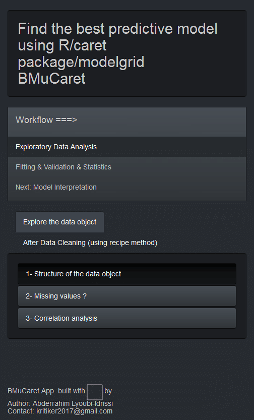
The BMuCaret Shiny Application

Conclusion

1. BMuCaret Shiny application should help reduce the effort made to perform comparison of caret models for a classification problem.
2. To use this application for a new data set the modules 1&2 need to be customised to the new classification problem.

Outlook

1. Implementing module1 and module2 into module3
2. Updating BMuCaret application to be also used for regression problems.
3. Implementing model interpretation(maybe with the lime package for R, or DALEX ..).
4. Developing a new Shiny application to perform model comparison by using other packages.
5. ….

Thank you in advance for your feedback.