Propagating nerve impulse in Hodgkin-Huxley model. Modeling with R. Part 1

The action potential is defined as the signal that is transmitted along an axon (also called nerve fiber). The axon is a portion of a nerve cell (neuron) that carries nerve impulses away from the cell body and enables nerve cells to communicate.
The scope of this article is to investigate the Hodgkin and Huxley (H&H) [1] model of a neuron’s action potential and the propagation of the action potential along the neuron’s axon.
In this blog we will use deSolve [2] R-package to solve the differential equations of the H&H model and the outputs of the simulation will be presented graphically, using the ggplot R library.

Biological Neuron

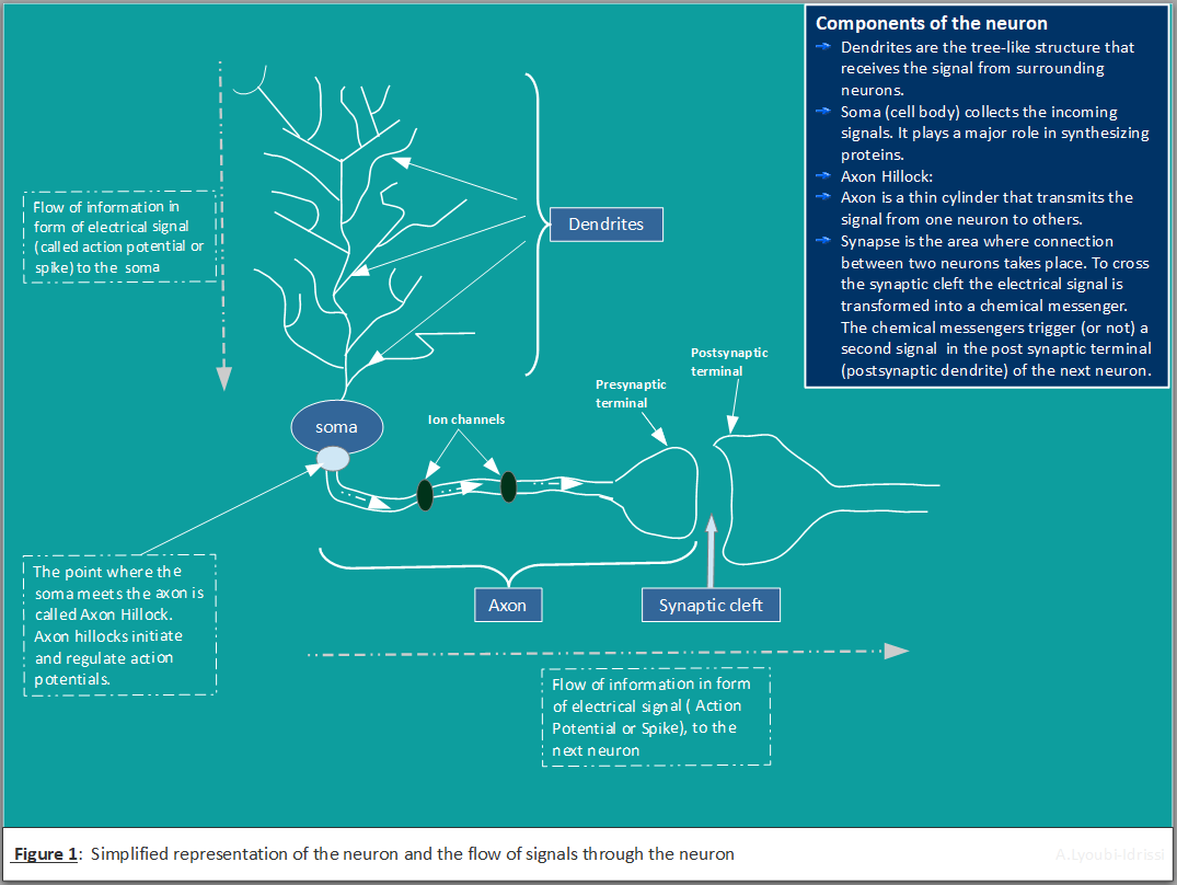
The primary characteristics of biological neural network is information processing.
Figure 1 shows a simplified representation of biological neuron and the corresponding signal propagation.

Ion Channels

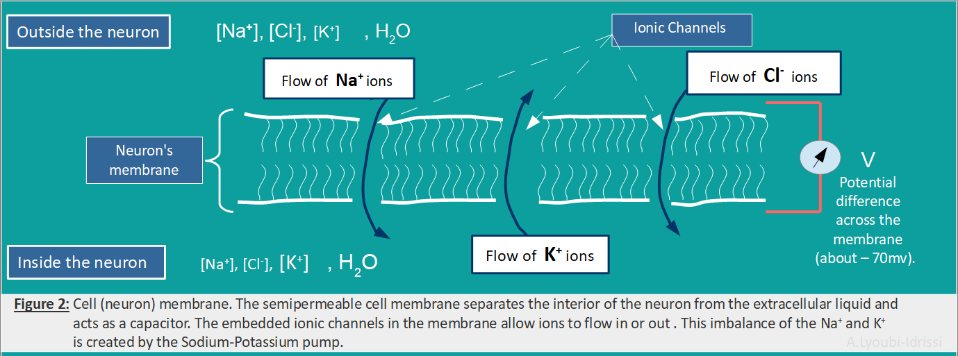
The core function of a neuron can be understood entirely in electrical terms: voltages (electrical potentials) and currents (flow of electrically charged ions in and out of the neuron membrane through tiny pores called ion channels). There are three main ions (Potassium, Sodium and Chloride) with different concentration outside and inside of the neuron (Figure2).

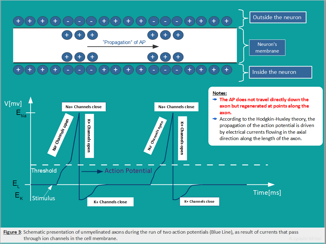
The movement of these ions through the ion channels (embedded in the neuron’s membrane) generates an electrical signal that is called an action potential (also referred as spike or nerve impulse).

Action Potential (Spike)

The action potential is the signal that is transmitted along an axon that enables nerve cells to communicate and to activate many different systems in an organism. Figure 3: Schematic representation of the action potential).

Hodgkin-Huxley Model

Hodgkin-Huxley (H&H) model is one of the most realistic and most important model in computational neuroscience. This model can be represented with the help of an electrical circuit and four equations (Figure 4). The neuronal membrane in the H&H model is considered as an electrical circuit involving a capacitor and three parallel series of batteries and variable resistors.

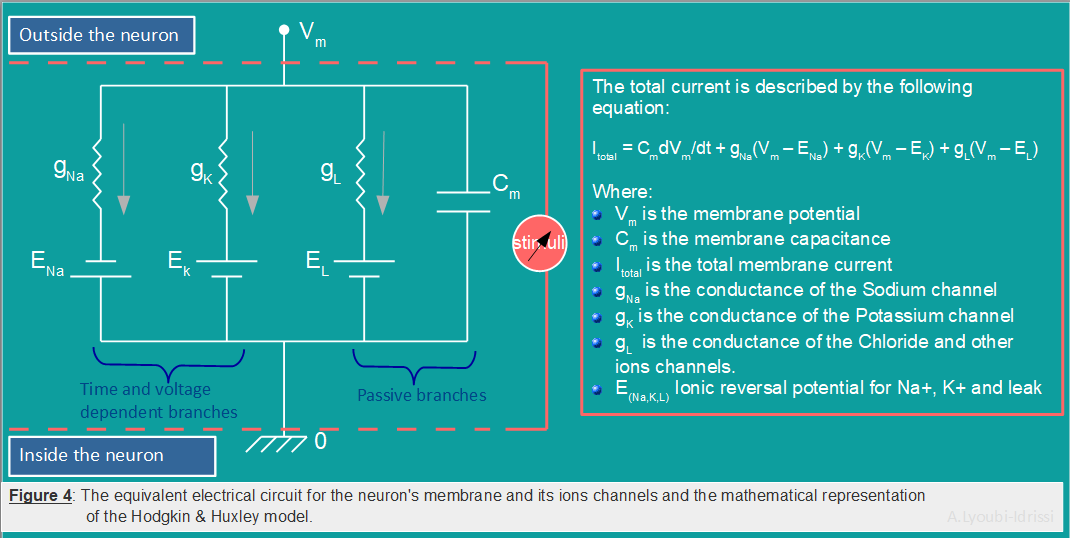
The total membrane current $I_m$ as a function of time and voltage is given by the following equation. The four terms on the right-hand side of $(H.1)$ give respectively the capacity current, the current carried by K ions, the current carried by Na ions and the leak current,
$$
\begin{align}
I_m = C_m\frac{\partial V_m}{\partial t} + I_{ion} \hspace{225pt} \\
I_m = C_m\frac{\partial V_m}{\partial t} + g_K(V_m -V_K)+g_{Na}(V_m – V_{Na}) + g_L(V_m – V_L) \hspace{20pt} (H.1)
\end{align}$$
Where:

$ C_m $ is the membrane capacitance

$V_{Na}$, $V_K$, $V_l$ are the ionic reversal potential for $Na^+$, $K^+$ and leak respectively.

$g_K = \bar{g}_K*n^4$ is the conductance of the potassium channel, and $\bar{g}_K$ is a constant and represents the maximum conductance value, and $n$ describes the activation.

$g_{Na} = \bar{g}_{Na}*m^3*h$ is the sodium conductance, and $\bar{g}_{Na}$ is a constant and represents the maximum conductance value; $m$ is the proportion of the sodium ion channels that are open (it represents the concentration of the Sodium(Na)). The combined action of $m$ and $h$ controls the sodium channels. The effective conductance of sodium channels is modeled as $1/RNa= \bar{g}_{Na}*m^3*h$, where $m$ describes the activation (opening) of the channel and $h$ its inactivation (blocking).

$g_L = constant$ is the leaky channel, which represents the concentration of various other ions.

The parameters that we are going to use for the simulations are those for the squid giant axon provided by Hodgkin & Huxley [A.L. Hodgkin and A.F. Huxley. A quantitative description of membrane current and its application to conduction and excitation in nerve. J. Physiol, 117:500–544, 1952.]. They are given by:
$$
\begin{align} C_m & \gets 1\ \mu\text{F}/\text{cm} \\ \bar{g}_{L} &\gets 0.3\ \text{mS}/\text{cm}^2 \\ V_{L} & \gets 10.613\ \text{mV} \\ \bar{g}_{K} & \gets 36\ \text{mS}/\text{cm}^2 \\ V_{K} &\gets -12\ \text{mV} \\ \bar{g}_{Na} &\gets 120\ \text{mS}/\text{cm}^2 \\ V_{Na} &\gets 115\ \text{mV} \end{align} $$
The dynamics of the dimensionless variables $m$, $n$ and $h$, which are gating variables describing the probability of ion channels being open, can be described by the following ordinary differential equations $(H.2)$, $(H.3)$, $(H.4)$:
$$
\frac{\partial n}{\partial t} = \alpha_n(1 – n) -\beta_nn \hspace{20pt} (H.2) \\
\: \frac{\partial m}{\partial t} = \alpha_m(1 – m) -\beta_mm \hspace{20pt} (H.3) \\
\frac{\partial h}{\partial t} = \alpha_h(1 – h) -\beta_hh \hspace{20pt} (H.4)
$$
The expressions of $\alpha ‘s$ and $\beta ‘s$ are given by the following equations $(H.5)$, $(H.6)$ and $(H.7)$.
$$
\alpha_n = \frac{0.01(10-V)}{\exp(\frac{10-V}{10})-1}, \hspace{20pt}\beta_n = 0.125\exp -\frac{V}{80} \hspace{20pt} (H.5)
$$ $$
\begin{align}
\alpha_m = \frac{0.1(25-V)}{\exp(\frac{25-V}{10})-1}, \hspace{20pt} \beta_m = 4\exp -\frac{V}{18} \hspace{20pt} (H.6)
\end{align}
$$ $$
\alpha_h = \frac{0.07}{\exp(-\frac{V}{20})}, \hspace{20pt} \beta_h = \frac{1}{1+ \exp\frac{30 – V}{10} }\hspace{20pt} (H.7)
$$
The appropriate numerical parameters in equations $(H.5), (H.6), (H.7)$ have been determined by experiment. Detailed description of the H&H model can be found in the original paper at here. A good introduction to the H&H model can be located here and here.

Solving ODEs of H&H Model using R-Package deSolve

The H&H model is mathematically complex, and has no analytical solution. Solving for the membrane action potential and the ionic currents requires integration approximated using numerical methods. Here we will use the the R-Package deSolve to solve the H&H differential equations and simulate the time evolution of the membrane potential and the dynamics of the gating variables $m$, $n$ and $h$.
The deSolve package is an add-on package of the open source data analysis system R for the numerical treatment of systems of differential equations.
The package contains functions that solve initial value problems of a system of first-order ordinary differential equations (ODE), of partial differential equations (PDE), of differential algebraic equations (DAE), and of delay differential equations (DDE).
The functions provide an interface to the FORTRAN functions lsoda, lsodar, lsode, lsodes of the ODEPACK collection, to the FORTRAN functions dvode, zvode, daspk and radau5, and a C-implementation of solvers of the Runge-Kutta family with fixed or variable time steps.
The package contains also routines designed for solving ODEs resulting from 1-D, 2-D and 3-D partial differential equations (PDE) that have been converted to ODEs by numerical differencing.

Steps to be taken

To implement and solve the H&H differential equations in R we proceed as follows: (Examples can be located at deSolve.)

Needed R-Packages

Load the required R-Packages

Model specification, which consists of:

Defining model parameters and their values,

Defining model state variables and their initial conditions,

Implementing the model equations that calculate the rate of change (e.g. $\frac {dx}{dt}$) of the state variables.

The model application, which consists of:

Specification of the time at which model output is wanted,

Integration of the model equations (uses R-functions from deSolve),

Plotting of model results and conducting correlation analysis and variable importance

So let’s now start with the R-coding.

Running the model and visualization of the results/outputs

The R-code to solve the H&H equations

## Code to study the H&H model
# Load required libraries
library(deSolve)
library(ggplot2)
library(dplyr)
library(see)
# Defining model parameters and their values
## Ena, Ek, El are ionic reversal potential for Na+, K+ and leak respectively
## C_m is the membrane capacitance
## gna, gk, gl are maximum conductance of sodium, potassium and leak respectively
## I is the applied current to the membrane(here it is set to 10 to have more than one spike)
parameters = c(Vna = 115, Vk = -12, Vl = 10.63, gna = 120, gk = 36, gl= 0.3, C = 1, I = 10)
## Set initial state
yini_2 <- c(V = -15, m = 0.052, h = 0.596, n = 0.317)
# Model equations(specified in the the following function sHH)
sHH <- function(time, y, parms) {
  with(as.list(c(y, parms)), {
## Ion channels functions/Gating functions
    alpha_m <- function(v) 0.1*(25-v)/(exp((25-v)/10)-1)
    beta_m  <- function(v) 4*exp(-v/18)
    alpha_h <- function(v) 0.07*exp(-v/20)
    beta_h  <- function(v) 1/(exp((30-v)/10)+1)
    alpha_n <- function(v) 0.01*(10-v)/(exp((10-v)/10)-1)
    beta_n  <- function(v) 0.125*exp(-v/80)
    # I <- 10*sin(0.5*time)
    # I <- 10*exp( -0.125*(time - 50)^2)
## Derivatives
    dV <- ( I - gna*h*(V-Vna)*m^3-gk*(V-Vk)*n^4-gl*(V-Vl))/C
    dm <- alpha_m(V)*(1-m)-beta_m(V)*m
    dh <- alpha_h(V)*(1-h)-beta_h(V)*h
    dn <- alpha_n(V)*(1-n)-beta_n(V)*n 
  list(c(dV, dm, dh, dn))
  })
}
# Model application
##Set integration times
time = seq(from =0, to=50, by = 0.01)
## Model integration (The model is solved using deSolve function ode, which is the default integration routine.)
## Running the model
print(system.time(
  out_sHH <- ode(yini_2 , func = sHH , times = time, parms = parameters)))
#Print the summary 
summary(out_sHH)

Plotting the results

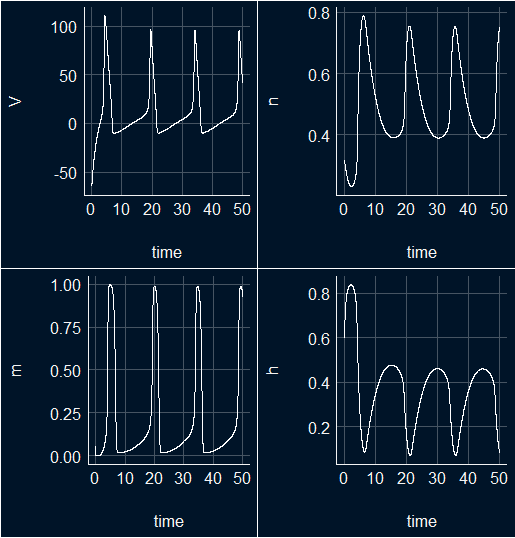
We transform the ode output to a data frame (s_HH_df) and use ggplot package to visualize the results. To visualize the variable importance we will use the MachineShop package to train the dataset and do the variable importance analysis.

s_HH_df <- as.data.frame(out_sHH)
pv <- ggplot(s_HH_df, aes(time,V)) + geom_line(color = "white") +  theme_abyss()
pn <- ggplot(s_HH_df, aes(time,n)) + geom_line(color = "white") +  theme_abyss()
pm <- ggplot(s_HH_df, aes(time,m)) + geom_line(color = "white") +  theme_abyss()
ph <- ggplot(s_HH_df, aes(time,h)) + geom_line(color = "white") +  theme_abyss()
ggpubr::ggarrange(pv, pn, pm, ph, ncol=2, nrow =2)

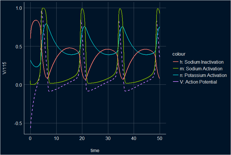
All in one plot

ggplot(s_HH_df, aes(x = time))+
  geom_line(aes(y = V/115, color ="V: Action Potential"),  lwd =1, linetype = 2)+
  geom_line(aes(y =n, color = "n: Potassium Activation"), lwd = 1)+
  geom_line(aes(y =m, color = "m: Sodium Activation"), lwd = 1)+
  geom_line(aes(y = h, color = "h: Sodium Inactivation"), lwd = 1)+
  theme_abyss()

All in one plot with animation.

The animated plot is showing the three main stages of the dynamical proprieties of the membrane potential and the gating functions in the H&H model: depolarization, repolarization, and hyperpolarization.

Here is code for the animation:

library(gganimate)
library(ggplot2)
library(gifski)
s_HH_df <- as.data.frame(out_sHH)
graph_3 <- ggplot(s_HH_df, aes(x = time))+
  geom_line(aes(y = V/115, color ="V: Action Potential"),  lwd =1, linetype = 2)+
  geom_line(aes(y =n, color = "n: Potassium Activation"), lwd = 1)+
  geom_line(aes(y =m, color = "m: Sodium Activation"), lwd = 1)+
  geom_line(aes(y = h, color = "h: Sodium Inactivation"), lwd = 1)+
  theme_abyss()
graph4.animation<- graph_3 +
  transition_reveal(time) +
  view_follow(fixed_y = TRUE)
animate(graph4.animation, height = 500, width = 800, fps = 90, duration = 10, start_pause = 80, end_pause = 60, res = 100)
# you should have a little patience :-)

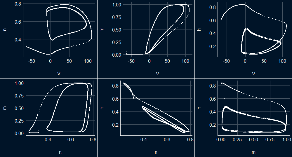
Phase diagrams

v_n <- ggplot(s_HH_df, aes(x=V, y = n)) + geom_point(color = "white", size = 0.3) + theme_abyss()
v_m <- ggplot(s_HH_df, aes(x=V, y = m)) + geom_point(color = "white", size = 0.3) + theme_abyss()
v_h <- ggplot(s_HH_df, aes(x=V, y = h)) + geom_point(color = "white", size = 0.3) + theme_abyss()
n_m <- ggplot(s_HH_df, aes(x=n, y = m)) + geom_point(color = "white", size = 0.3) + theme_abyss()
n_h <- ggplot(s_HH_df, aes(x=n, y = h)) + geom_point(color = "white", size = 0.3) + theme_abyss()
m_h <- ggplot(s_HH_df, aes(x=m, y = h)) + geom_point(color = "white", size = 0.3) + theme_abyss()
ggpubr::ggarrange(v_n, v_m, v_h, n_m, n_h, m_h, ncol=3, nrow =2)

Performing correlation analysis

Two R-tools will be used to perform correlation analysis and visualizing the relationships between the H&H model´s parameters in the produced data set s_HH_df; Gaussian graphical model and Heatmap.

Gaussian graphical model

library(correlation)
library(see) # for plotting
library(ggraph)
library(dplyr)
s_HH_df % 
  correlation(partial = TRUE) %>% 
  plot()

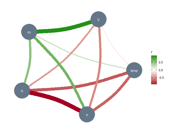
The thickness of the lines represents the strength of the relationships between the variables. The absence of a line implies no or very weak relationships between the relevant variables. In the Gaussian graphical model, these lines capture partial correlations, that is, the correlation between two variables when controlling for all other variables included in the data set (s_HH_df). Note the relationship (line thickness) between the membrane potential $V$ and the sodium activation variable $m$, and between $n$ and $h$. These results are confirmed below, where we have used another correlation tool.

Heatmap

library(corrplot)
library(RColorBrewer)
M <-cor(s_HH_df)
corrplot(M, method="number", type = "upper")

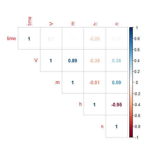
The plot above shows a highly significant positive correlation between $V$ and $m$ and a significant negative correlation between $n$ and $h$.

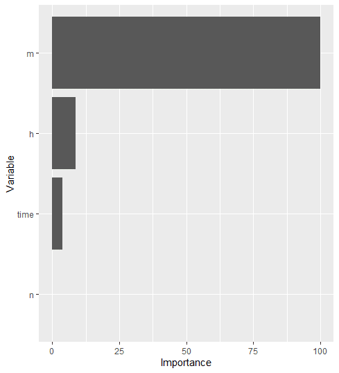
Variable importance

MachineShop package is used to train the dataset (s_HH_df) and do the variable importance analysis.

## Analysis libraries
library(MachineShop)
library(ggplot2)
## Training and test sets
set.seed(123)
train_indices <- sample(nrow(s_HH_df), nrow(s_HH_df) * 2 / 3)
trainset <- s_HH_df[train_indices, ]
testset <- s_HH_df[-train_indices, ]
## Model formula
fo <- V ~ .
## Boosted regression model tuned with the training set
model_fit % fit(fo, data = trainset)
## Variable importance
vi <- varimp(model_fit)
plot(vi)

Houtlook

H&H model is one of the most realistic and most important model in computational neuroscience. H&H used the voltage clamp technique to measure the kinetics of $Na^+$ and $K^+$ currents in the squid giant axon. They have build a set of differential equations that describe the dynamics of the action potential. Furthermore, by combining these equations with the cable equation for spreading of the current in the axon they were able to calculate the shape and velocity of the propagating action potentials. In part1 of this blog we used the H&H differential equations to model the neuronal electrical activity. We solved the model differetial equations by using the deSolve R-Package. In the second part of this blog we will investigate the mechanisms of the propagation of nerve activity and present mathematical models, which describe the signal propagation in nerve fibers. There we will again make use of the deSolve R-package to solve the so called passive and active cable equations.

References

[1] Hodgkin AL, Huxley AF. (1952) “A quantitative description of membrane current and its application to conduction and excitation in nerve”. The Journal of Physiology. 117 (4): 500-544, August 1952.
[2] Soetaert K, Petzoldt T, Setzer RW (2010). “Solving Differential Equations in R: Package deSolve.” Journal of Statistical Software, 33(9), 1–25. ISSN 1548-7660, doi: 10.18637/jss.v033.i09,

Hodgkin & Huxley modelNerve Pulse TransmissionNeuron Modeling