In this post, the failure pressure will be predicted for a pipeline containing a defect based solely on burst test results and learning machine models. For this purpose, various Machine Learning models will be fitted to test data under R using the caret package, and in the process compare the accuracy of the models in order to identify the best performing one(s).
Importing The Data
The data set to be used, has been extracted from an extensive database of burst test results, the set contains the results of approximately 313 tests which were compiled by GL in 2009. Report as well as the data used here can be obtained using this link.
The data was extracted and inserted into a CSV file, allowing for it to be called and manipulated easily.
Data used in this tutorial can be found in this file.
We will start by loading all libraries needed to run the analysis and the data set.
library(caret)
library(caretEnsemble)
library(ggforce)
library(ggplot2)
library(gridExtra)
Burst_Tests_Data <- read.csv(file="F:/kamel/Burst Data.csv", header=TRUE, sep=",")
# Summary of the data is shown below:
  summary(Burst_Tests_Data)
##        INDEX              Source_Reference     Grade       OD_by_WT
##  INDEX 1  :  1   BRITISH GAS RING1:  1     X52    :58   Min.   :  8.60
##  INDEX 10 :  1   BRITISH GAS RING2:  1     B      :50   1st Qu.: 46.20
##  INDEX 100:  1   BRITISH GAS RING3:  1     X60    :46   Median : 57.90
##  INDEX 101:  1   BRITISH GAS RING4:  1     X65    :44   Mean   : 58.77
##  INDEX 102:  1   BRITISH GAS RING5:  1     X100   :41   3rd Qu.: 70.70
##  INDEX 103:  1   BRITISH GAS RING6:  1     X46    :41   Max.   :111.10
##  (Other)  :307   (Other)          :307     (Other):33
##    Defect_Type   Norm_Length         d_by_WT        YS_by_SMYS
##  Machined:180   Min.   :  0.228   Min.   :0.089   1.134  : 41
##  Real    :133   1st Qu.:  1.594   1st Qu.:0.448   N/A    : 19
##                 Median :  3.549   Median :0.586   1.194  : 17
##                 Mean   : 36.323   Mean   :0.567   1.117  : 11
##                 3rd Qu.:  9.878   3rd Qu.:0.715   1.211  : 10
##                 Max.   :284.164   Max.   :1.000   1.092  :  9
##                                                   (Other):206
##   UTS_by_SMTS    YS_by_UTS   Failure_Mode Failure_Pressure_psi
##  N/A    : 62   N/A    : 62   L  : 79      Min.   :  677
##  1.057  : 41   0.976  : 41   N/A: 73      1st Qu.: 1434
##  1      : 18   0.634  : 17   R  :161      Median : 1844
##  1.098  : 17   0.771  : 10                Mean   : 2252
##  1.045  :  9   0.773  : 10                3rd Qu.: 2363
##  1.048  :  9   0.834  :  9                Max.   :17999
##  (Other):157   (Other):164
##  Failure_Pressure_Mpa      SMYS            SMTS
##  Min.   :  4.668      Min.   :172.0   Min.   :310.0
##  1st Qu.:  9.887      1st Qu.:317.0   1st Qu.:434.0
##  Median : 12.714      Median :359.0   Median :455.0
##  Mean   : 15.525      Mean   :398.3   Mean   :505.1
##  3rd Qu.: 16.292      3rd Qu.:448.0   3rd Qu.:531.0
##  Max.   :124.099      Max.   :689.0   Max.   :757.0
##
Prepare Dataset
The main parameters needed for the analysis will be separated from the loaded data and into another set, the main parameters we need are:
- Normalised length
- Diameter to wall thickness ratio
- Defects depth
- Burst Pressure
- SMYS
- Failure Mode (for visualisation)
Data <- data.frame(Norm_L = Burst_Tests_Data$Norm_Length, Depth = Burst_Tests_Data$d_by_WT, OD_by_WT = Burst_Tests_Data$OD_by_WT, SMYS = Burst_Tests_Data$SMYS, Test_P_Burst = Burst_Tests_Data$Failure_Pressure_Mpa, Failure_Mode=Burst_Tests_Data$Failure_Mode)
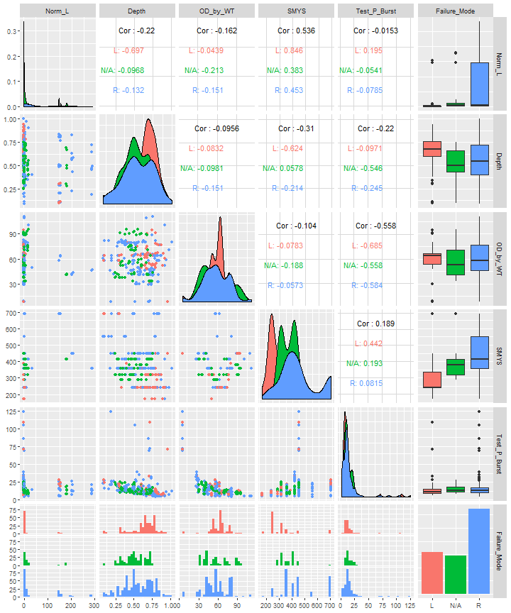
We can view all of the selected parameters using pairwise comparison on the basis of the failure mode.
library(GGally)
ggpairs(Data, mapping = aes(color = Failure_Mode))
Next step is to partition our data into 2 sets, 90% for training and 10% for testing, these will be balanced splits based on the burst pressure values. The purpose of splitting the data is to allow the algorithms to learn the relationships between the parameters with the training set, followed by the testing set, which will be used as an independent set to make sure our trained model is not over-fitting the data during the training step.
Split_Data <- createDataPartition(Data$Test_P_Burst, p = 0.90, list = FALSE)
Training_Data <- Data[Split_Data,]
Testing_Data <- Data[-Split_Data,]
Train the Models
There is a large list of machine learning algorithm supported by the caret package; however, for this analysis, I chose randomly 6 regression models, these are:
- Model Tree
- Support Vector Machines with Linear Kernel
- Random Forest
- k-Nearest Neighbors
- Generalized Linear Model
- Projection Pursuit Regression
We will use repeated cross-validation which is a way to evaluate the performance of a model by randomly partitioning the training set into k equal size subsamples. Of the k subsamples, a single subsample is retained as the validation data for testing the model, and the remaining k-1 subsamples are used as training data. The cross-validation process is then repeated k times, for our analysis we will use 10 folds and 10 repeats.
Each of the 6 models will be built using the function 'train()', the relationship between parameters will be expressed as follow:
Purst Pressure = f(Normalised Length, Depth, OD/WT, SMYS)
At the end, we will use the 10% testing data to predict the burst pressure for each trained model, using the function 'predict()'.
train.control <- trainControl(method = "repeatedcv", number = 10, repeats = 10, verboseIter=FALSE)
Formula <- Test_P_Burst ~ Norm_L + Depth + OD_by_WT + SMYS
Test_Data <- subset(Testing_Data , select = c("Norm_L", "Depth", "OD_by_WT", "SMYS"))

# Model Rules
Model_MR <- train(Formula, data = Training_Data, method = "M5Rules", trControl = train.control, preProc = c("center", "scale"))
Model_MR_P_Burst <- predict(Model_MR, Testing_Data)

# Support Vector Machines with Linear Kernel
Model_SVM <- train(Formula, data = Training_Data, method = "svmLinear", trControl = train.control, tuneGrid = expand.grid(C = c(0.01, 0.1, 0.5)), preProc = c("center", "scale"))
Model_SVM_P_Burst <- predict(Model_SVM, Testing_Data)

# Random Forest
Model_RF <- train(Formula, data = Training_Data, method = "rf", trControl = train.control, ntree=200, preProc = c("center", "scale"))
Model_RF_P_Burst <- predict(Model_RF, Testing_Data)

# k-Nearest Neighbors
Model_KNN <- train(Formula, data = Training_Data, method = "knn", trControl = train.control, tuneLength = 10, preProc = c("center", "scale"))
Model_KNN_P_Burst <- predict(Model_KNN, Testing_Data)

# Generalized Linear Model
Model_GLM <- train(Formula, data = Training_Data, method = "glm", trControl = train.control, tuneLength = 10, preProc = c("center", "scale"))
Model_GLM_P_Burst <- predict(Model_GLM, Testing_Data)

# Projection Pursuit Regression
Model_PPR <- train(Formula, data = Training_Data, method = "ppr", trControl = train.control, tuneLength = 10, preProc = c("center", "scale"))
Model_PPR_P_Burst <- predict(Model_PPR, Testing_Data)

Models <- resamples(list(MR = Model_MR, RF = Model_RF, SVM = Model_SVM, KNN = Model_KNN, GLM = Model_GLM, PRR = Model_PPR))
Compare the Models
Now we have trained and tested all of our 6 models, let's have a look at how each model performed. First plot of the predicted burst pressure Vs. the real burst pressure:
library(ggthemes)
Test_Failure_P <- Testing_Data$Test_P_Burst
Markers <- geom_point(size=1.5, shape=6, color="black")
Unity <- geom_abline(slope=1, intercept = 0, color="red", linetype="dashed",size=1)
Bground <- theme(axis.title = element_text(face="bold", size=12), panel.background = element_rect(fill = 'lightsteelblue4'), panel.grid = element_line(colour="grey"), plot.background=element_rect(fill="grey95"))
P1 <- ggplot(,aes(x = Test_Failure_P, y = Model_MR_P_Burst)) + Markers + Unity + Bground
P2 <- ggplot(,aes(x = Test_Failure_P, y = Model_SVM_P_Burst)) + Markers + Unity + Bground
P3 <- ggplot(,aes(x = Test_Failure_P, y = Model_RF_P_Burst)) + Markers + Unity + Bground
P4 <- ggplot(,aes(x = Test_Failure_P, y = Model_KNN_P_Burst)) + Markers + Unity + Bground
P5 <- ggplot(,aes(x = Test_Failure_P, y = Model_GLM_P_Burst)) + Markers + Unity + Bground
P6 <- ggplot(,aes(x = Test_Failure_P, y = Model_PPR_P_Burst)) + Markers + Unity + Bground
grid.arrange(P1, P2, P3, P4, P5, P6, nrow=2)
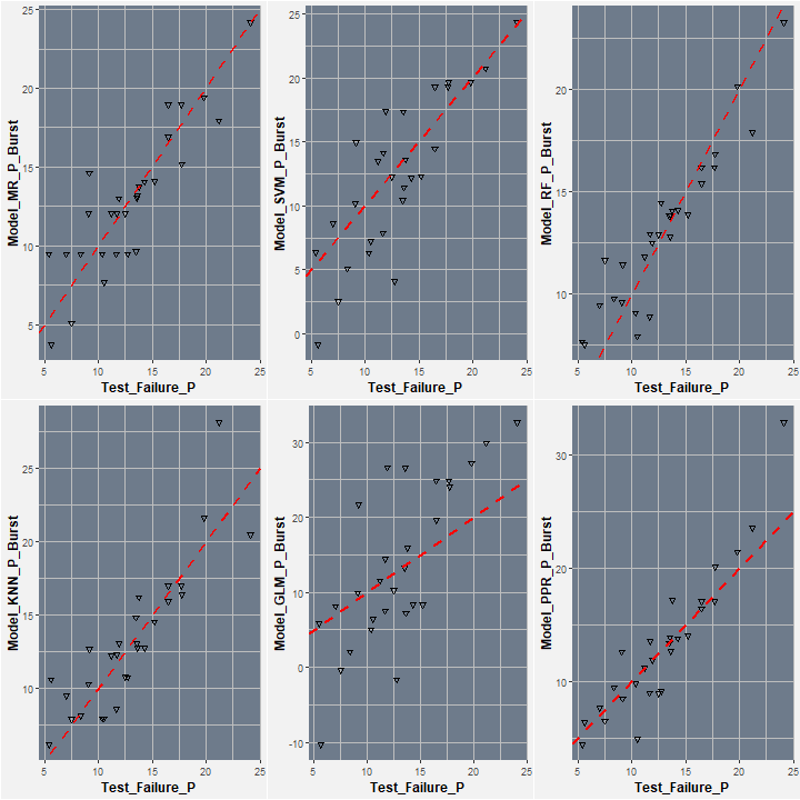
We can see that in overall, the Random Forest appears to be the most accurate model, however, performance is not totally that clear from the plots alone, for a clear comparison we can use some evaluation metrics, these can be viewed by calling the function summary().
summary(Models)
##
## Call:
## summary.resamples(object = Models)
##
## Models: MR, RF, SVM, KNN, GLM, PRR
## Number of resamples: 100
##
## MAE
##         Min.  1st Qu.   Median     Mean  3rd Qu.      Max. NA's
## MR  1.249353 1.961890 2.341977 2.611588 3.200767  5.861817    0
## RF  1.023035 1.495052 1.728636 1.908296 2.125849  4.333484    0
## SVM 1.986233 2.777073 3.766255 4.289719 5.560249 10.508175    0
## KNN 1.133630 1.858979 2.138108 2.655981 3.050784  6.585347    0
## GLM 3.070781 4.524447 5.415050 5.652634 6.456241 10.905213    0
## PRR 1.167177 1.861359 2.260386 2.293145 2.678526  3.878608    0
##
## RMSE
##         Min.  1st Qu.   Median     Mean   3rd Qu.      Max. NA's
## MR  1.557999 2.623602 3.619572 4.472389  5.756353 14.857580    0
## RF  1.227453 2.092623 2.482315 3.415498  3.719935 11.558717    0
## SVM 2.487095 3.660816 8.935002 9.425596 16.255103 25.082527    0
## KNN 1.491673 2.677945 3.185990 5.282331  6.621437 20.164751    0
## GLM 3.721669 5.943858 7.765995 9.409684 12.624701 22.397631    0
## PRR 1.550538 2.596583 3.350004 3.793293  4.563330  9.107361    0
##
## Rsquared
##             Min.   1st Qu.    Median      Mean   3rd Qu.      Max. NA's
## MR  0.0002491479 0.8188490 0.8872148 0.8464541 0.9523463 0.9863039    0
## RF  0.7559770108 0.9101539 0.9545877 0.9344962 0.9787224 0.9939840    0
## SVM 0.2365625650 0.4314300 0.5670594 0.5446240 0.6590483 0.8127915    0
## KNN 0.5504808103 0.7854814 0.8823773 0.8547489 0.9483226 0.9844278    0
## GLM 0.3281077690 0.4974465 0.5495725 0.5538143 0.6003874 0.8050598    0
## PRR 0.6472502237 0.8316454 0.9302789 0.8939118 0.9687244 0.9913075    0
We can also compare the accuracy of the models visually by using the dot plot.
scales <- list(x=list(relation="free"), y=list(relation="free"))
dotplot(Models, scales=scales, layout=c(3,1))
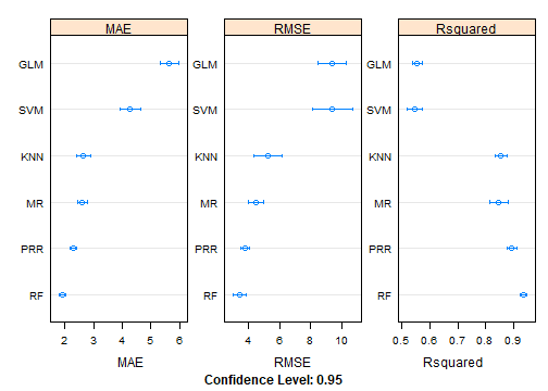
It is clear from the above, Random Forst appears to be the optimal model in this analysis, now we can use it in a normal assessment.
First let’s have a look how normal defect assessment method perform when compared to the test data (in this case I have selected the Modified ASME B31G method). For that, we create a function to calculate burst pressure of the defects used in the tests and add results to the parameters we selected previously.
# Modified ASME B31G
P_Burst <- function(Norm_Length, d_by_WT, OD_by_WT, SMYS){
if (Norm_Length <= 50^0.5)
{
    M <-  (1 + 0.6275*Norm_Length - 0.003375*Norm_Length^2)^0.5
} else {
    M <-  0.032*Norm_Length + 3.3
}
Sig_Flow <- SMYS + 69
P <- (((2*Sig_Flow)/OD_by_WT )*(1-0.85*d_by_WT))/(1-((0.85*d_by_WT)/M))
return(P)
}

# Calculate burst pressure for test defects
B31G_P_Burst <- c()
for(i in 1:length(Burst_Tests_Data[,1]))
{
  B31G_P_Burst[i] <- P_Burst(Burst_Tests_Data$Norm_Length[i], Burst_Tests_Data$d_by_WT[i], Burst_Tests_Data$OD_by_WT[i], Burst_Tests_Data$SMYS[i])
}

# Add results to previous selection
Data <- data.frame(Norm_L = Burst_Tests_Data$Norm_Length, Depth = Burst_Tests_Data$d_by_WT, OD_by_WT = Burst_Tests_Data$OD_by_WT, SMYS = Burst_Tests_Data$SMYS, Test_P_Burst = Burst_Tests_Data$Failure_Pressure_Mpa, B31G_P_Burst)
Let’s have a look how Modified B31G burst pressure results compare to tests results.
P <- ggplot(Data, aes(x = Test_P_Burst, y = B31G_P_Burst))+ geom_point(size=1.6, shape=6, colour = "black")+
labs(x = "Test Burst Pressure", y = "Modified B31G Burst Pressure") +
geom_abline(aes(slope=1, intercept = 0), linetype="dashed", size=1, colour = "red")+
theme(panel.background = element_rect(fill = 'lightsteelblue4'),
      axis.title = element_text(face="bold", size=12),
      plot.background=element_rect(fill="white"),
      axis.text = element_text(colour = "black", size=11))
P + facet_zoom(x = Test_P_Burst < 40, y = B31G_P_Burst < 40, horizontal=F,zoom.size = 1)
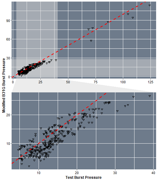
We can see that in overall, the Modified B31G tend to under-estimate the values of the burst pressure. Now let's have a practical test with a new data set, created randomly.
Rep_Nb <- 500    # Random numbers to be genrated
L <- runif(Rep_Nb, min=5, max=100)
dt <- runif(Rep_Nb, min=0.1, max=0.7)
OD <- rep(406.4, times=Rep_Nb)
SMYS <- rep(359, times=Rep_Nb)
WT <- runif(Rep_Nb, min=5, max=15)
Norm_L <- L/(OD*WT)^0.5
OD_by_WT <- OD/WT
Depth <- dt

# Now let's predict the burst pressure using the best performing model, i.e. neural networks.
Pract_Test <- data.frame(Norm_L, Depth, OD_by_WT, SMYS)
Pract_P_Burst <- predict(Model_RF, Pract_Test)

# Estimate the burst pressure of the randomly generated parameters using Modified B31G
B31G_P_Pract <- c()
for(i in 1:Rep_Nb)
{
 B31G_P_Pract[i] <- P_Burst(Norm_L[i], Depth[i], OD_by_WT[i], SMYS[i])
}
ggplot(, aes(x = Pract_P_Burst, y = B31G_P_Pract))+ geom_point(size=1.6, shape=6, colour = "black")+
labs(x = "Predicted Pressure", y = "Modified B31G Pressure") +
geom_abline(aes(slope=1, intercept = 0), linetype="dashed", size=1, colour = "red")+
theme(panel.background = element_rect(fill = 'lightsteelblue4'),
      axis.title = element_text(face="bold", size=12),
      plot.background=element_rect(fill="white"),
      axis.text = element_text(colour = "black", size=11))
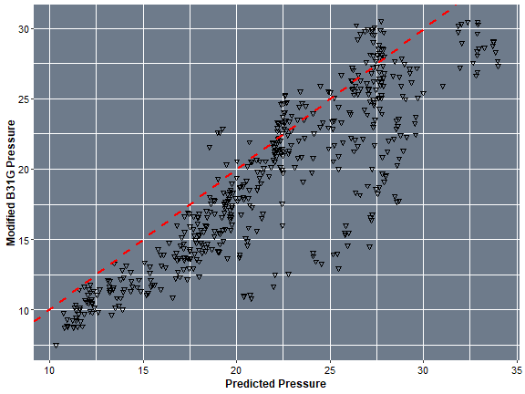
In The above guide we only limited the number of models to 6; however, we can include as many as we want for better selection. In the next post, I will be showing how to combine multiple models as an ensemble for better predictions.
Hi KT !
I would apreciate if you can provide me the post about how to combine multiple models as an ensemble for better predictions.
Thanks in advance !
Javier
Hi Javier,
I will be working the subject and hopefully will be posted soon.
Regards,
Kamel
Hi, how can get csv file to test the code? Extracted data I mean
Hi Rustu,
I have not included the csv file, but you can always extract the data from the PDF document which you can access through I included in text. I will try in next few days to upload the file.
Thanks, will look for it.
Hi Rustu,
Link to file is below
https://ufile.io/scqak
Hi ,
above link is not working can you please share .csv file again
Hi,
please find new link below
https://ufile.io/xhzf4
Hey KT,
Sorry to say but above link is also not working/ not opening can you please upload file on github or maybe on Kaggle and provide link of the same it will be helpful for me
Hi,
To make it easy, I have attached the file in the post itself at the start, let me know if you have a problem.