In this paper, we will go through the MBA (Market Basket analysis) in R, with focus on visualization of MBA. We will use the Instacart customer orders data, publicly available on Kaggle. The dataset is anonymized and contains a sample of over 3 million grocery orders from more than 200,000 Instacart users.
MBA is a modeling technique based on the theory that if you buy a certain group of items, you are more (or less) likely to buy another group of items. For example, it may be possible that people who buy milk, also likely to buy a banana (because most of them are planning on making banana milkshake). The set of items a customer buys is referred to as an item set, and MBA seeks to find relationships between purchases.
Typically, the relationship will be in the form of a rule:
IF {milk} THEN {banana}.
The probability that a customer will buy milk (i.e. that LHS of the rule is true) is referred to as the support for the rule. The conditional probability that a customer will purchase banana is referred to as the confidence.
In general, Support is the basic probability of an event to occur. If we have an event to buy product A, Support(A) is the number of transactions which includes A divided by the total number of transactions. The confidence of an event is the conditional probability of the occurrence; the chances of A happening given B has already happened. Lift is the ratio of confidence to expected confidence. The probability of all of the items in a rule occurring together (otherwise known as the support) divided by the product of the probabilities of the items on the left and right side occurring as if there was no association between them. The lift value tells us how much better a rule is at predicting something than randomly guessing. The higher the lift, the stronger the association.
Apriori algorithm was used for frequent itemset mining and association rule learning over transactional databases. It proceeds by identifying the frequent individual items in the database and extending them to larger and larger item sets as long as those itemsets appear sufficiently often in the database. The frequent itemsets determined by Apriori can be used to determine association rules which highlight general trends in the database.
There is a arules package” in R which implements the apriori algorithm can be used for analyzing the customer shopping basket. It requires 2 parameters to be set which are Support and Confidence.
We will see how Market Basket analysis performed propose recommendations in 2 areas: Store Layout & Marketing and Catalogue Arrangement.
Data Preparation
Our goal was to identify associated products. The first step before implementing Apriori algorithm is data preparation, consisting of following steps:
- Creating customer shopping basket, where each row is ordered id and have a list of products purchased in that order.
- The shopping basket was then converted to transaction data, where each order is one transaction.
- Order ID was used as transaction ID and Product names as a target for Apriori algorithm.
- Summary of the transaction shows that most frequently bought an item is banana and one transaction may have one, two or more than 2 items purchased.
# Load packages
library(data.table)
library(dplyr)
library(ggplot2)
library(knitr)
library(stringr)
library(DT)
library(plotly)
library(arules)
library(arulesViz)
library(visNetwork)
library(igraph)
library(kableExtra)
# Load data files
order_products_train <- fread('order_products_train.csv')
products <- fread('products.csv')
# Create Shopping basket:
order_baskets=order_products_train %>%
inner_join(products, by="product_id") %>%
group_by(order_id) %>%
summarise(basket = as.vector(list(product_name)))

# Create transaction data
transactions <- as(order_baskets$basket, "transactions")
inspect(transactions[1])
items
[1] {Bag of Organic Bananas,
     Bulgarian Yogurt,
     Cucumber Kirby,
     Lightly Smoked Sardines in Olive Oil,
     Organic 4% Milk Fat Whole Milk Cottage Cheese,
     Organic Celery Hearts,
     Organic Hass Avocado,
     Organic Whole String Cheese}
The output above shows that one transaction contains list of products.
Implement Apriori Algorithm
Parameters while generating rules were: Support=0.005, Confidence=0.25
Among generated rules, there were some repeated or redundant rules (for instance, one rule is the super rule of another rule), so they were pruned. There were total 27 rules, after pruning. The First rule tells that if customer buy Organic Cilantro, they are 6.21 times more likely to buy Limes, compared to random. The Top 5 rules are shown below:
# Implementing Apriori Algorithm
rules <- apriori(transactions, parameter = list(support = 0.005, confidence = 0.25))

# Remove redundant rule
rules <- rules[!is.redundant(rules)]
rules_dt <- data.table( lhs = labels( lhs(rules) ),
                        rhs = labels( rhs(rules) ),
                        quality(rules) )[ order(-lift), ]
head(rules_dt,5)
lhs                      rhs     support confidence     lift count
1:                            {Organic Cilantro}                  {Limes} 0.007674778  0.2855927 6.211228  1007
2:                                       {Limes}            {Large Lemon} 0.012156178  0.2643792 4.264159  1595
3:   {Organic Hass Avocado,Organic Strawberries} {Bag of Organic Bananas} 0.005411214  0.4613385 3.910321   710
4:                         {Organic Raspberries}   {Organic Strawberries} 0.012727785  0.3011179 3.626710  1670
5: {Bag of Organic Bananas,Organic Hass Avocado}   {Organic Strawberries} 0.005411214  0.2933884 3.533615   710
Interpretation & Analysis
It is important to identify which products were sold how frequently in our dataset. Let’s analyze the associations with the help of visualization.
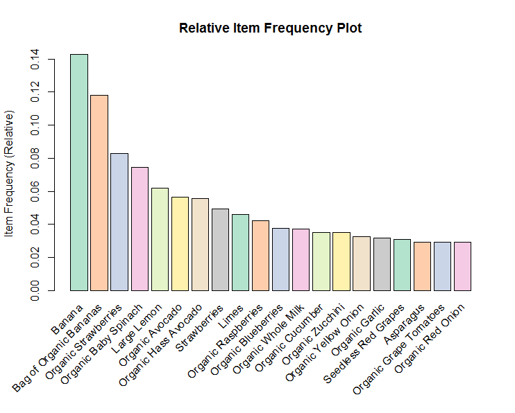
Item Frequency Plot
Item Frequency Histogram tells how many times an item has occurred in our dataset as compared to the others. The relative frequency plot shows that “Banana” and “Bag of Organic Banana” constitute around 1/4th of the transaction dataset; 1/4th the total sales are these items. It means that many people are buying these items.
So, Other items can be placed on the more frequently purchased items to boost the sales, for instance Organic Grape tomatoes can be placed beside Banana and Bag of Organic Banana.
library("RColorBrewer")
arules::itemFrequencyPlot(transactions,
   topN=20,
   col=brewer.pal(8,'Pastel2'),
   main='Relative Item Frequency Plot',
   type="relative",
   ylab="Item Frequency (Relative)")
Gives this plot:
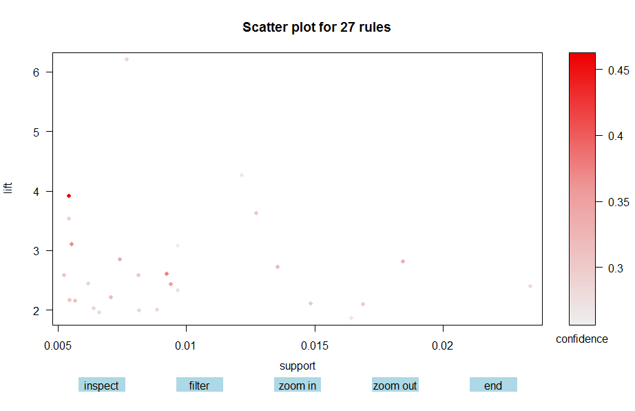
Scatter Plot
Rules with high lift have typically a relatively low support.
plotly_arules(rules)
Gives this plot:
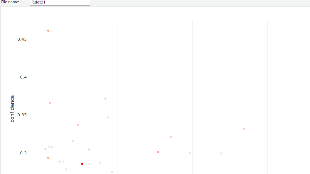
Interactive Scatterplot
Scatter plot method offers interactive features for selecting and zooming.Interaction is activated using interactive=TRUE.
Interactive features include:
- Inspecting individual rules by selecting them and clicking the inspect button.
- Inspecting sets of rules by selecting a rectangular region of the plot by inspecting button.
- Zooming into a selected region (zoom in/zoom out buttons).
- Filtering rules using the measure used for shading by clicking the filter button and selecting a cut-off point in the color key.
sel <- plot(rules, measure=c("support", "lift"),
          shading = "confidence",
          interactive = TRUE)
Gives this plot:
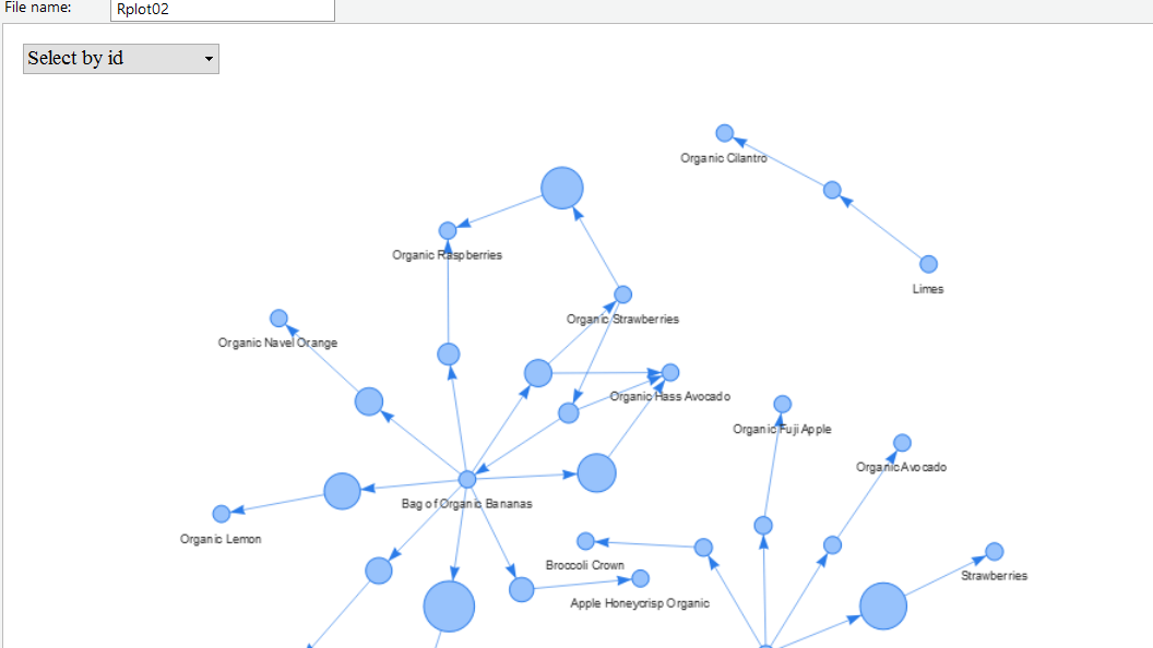
Network graph Visualisation
In this Vis each node rethe presents product in shopping basket and each rule from ==> to is an edge of the graph. The graphs tells that if a customer buys Bag of Organic banana. He is likely to buy Organic Lemon, Organic Large Extra Fancy Fuji Apple ..etc.
subrules2 <- head(sort(rules, by="confidence"),20)
ig <- plot( subrules2, method="graph", control=list(type="items") )
ig_df <- get.data.frame( ig, what = "both" )
nodesv %>%
   visNodes(size = 10) %>%
   visLegend() %>%
   visEdges(smooth = FALSE) %>%
   visOptions(highlightNearest = TRUE, nodesIdSelection = TRUE) %>%
   visInteraction(navigationButtons = TRUE) %>%
   visEdges(arrows = 'from') %>%
   visPhysics(
        solver = "barnesHut",
        maxVelocity = 35,
        forceAtlas2Based = list(gravitationalConstant = -6000)
      )
Gives this plot:
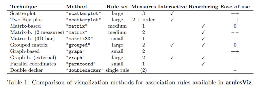
There are many other visualization techniques available in arulesViz package to understand the association rules. Below is the comparison of visualization methods for association rules available in arulesViz:
Conclusion
At last, we will see how these rules can help in-store layout and catalog arrangement. As we know that Instacart is a web app and in web analytics, data reflects the way users behave, and the way they are encouraged to behave, by the website design decisions earlier made. Market Basket analysis can be used to drive bussiness decision making by using the association results. There are a number of ways in which MBA can be used:
Associated Aisles should be placed together on the web application platform to boost the sales and reduce the time spent in finding that Aisle. For instance, cereal, lunch meat, and Bread Aisle should be placed together, as they are highly associated.( you can generate this rule by using aisle names in transaction data-set instead of product names while preparing data for Apriori algorithm)
Associated products such as Organic Cilantro and limes should be put close to one another, to improve the customer shopping experience and improving the store layout.Marketing can take benefit from this association relationship, for example, target customers who buy Organic Cilantro with offers of Lime, to encourage them to spend more on their shopping basket.
List of rules can be used to put recommendations on the product pages and at product cart pages.Those rules that are applicable to each product with the high lift where the product recommended has a high margin should be considered.It can drive the significant uplift in profit.
Hope you all liked the article.Let me know your thoughts on this.
Make sure to like & share it. Cheers!