Hope you liked the Part 1 ,Part 2 and Part 3 of this Series. In this Part 4, we will go through the tools used during the Improve phase of Six Sigma DMAIC cycle. The most representative tool used during the Improve Phase is DOE-Design of experiments. Proper use of DOE can lead to process improvement, but a bad design of experiment can lead to undesired results – inefficiency, higher costs.
What is experiment
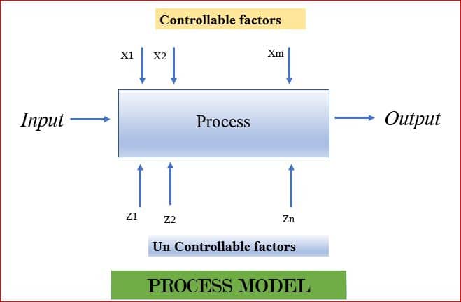
An experiment is a test or series of tests in which purposeful changes are made to input variables of a process or system so that we may observe and identify the reason for the change in output response.
Consider the example of the simple process model, shown below, where we have controlled input factors X’s, output Y and uncontrolled factors Z’s.
The objective of the experiment can be:
- Process Characterization: To know the relationship between X, Y & Z.
- Process Control: Capture changes in X, so that Y is always near the desired nominal value.
- Process Optimization: Capture changes in X, so that the variability of Y is minimized.
- Robust Design: Capture changes in X, so that effect of uncontrolled Z is minimized.
Importance of experiment
Experiments allow to control the values of the Xs of the process and then measure the value of the Ys to discover what values of the independent variables will allow us to improve the performance of our process. On the contrary, in the case of Observational Studies, we don’t have any influence on the variables we are measuring. We just collect the data and use the appropriate statistical technique.
There are some risks associated when the analysis is based on the data gathered directly during the normal performance of process: Inconsistent Data, Variable Value Range ( performance of X’s outside range not known ) & Correlated Variables.
Characteristics of well planned experiments
Some of the Characteristics of well-planned experiments are:
- The degree of Precision:
Probability should be high that experiment will be able to measure the differences with a degree of precision the experimenter desires. It implies appropriate design and sufficient replication. - Simplicity:
As simple as possible consistent with the objectives of experiment. - The absence of Systematic Error:
Units receiving one treatment should not differ in any systematic way from those receiving other treatment. - The range of Validity of Conclusions:
Experiments replicated in time and space would increase the range of validity of conclusions. - Calculation of the degree of Uncertainty:
A possibility of obtaining the observed results by chance alone.
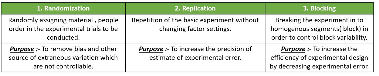
Three basic principle of Experiments
Three basic principles of experiments are Randomization, Repetition & Blocking.
Lets understand this through an example – A food manufacturer is searching for the best recipe for its main product: a pizza dough. The managers decided to perform an experiment to determine the optimal levels of the three main ingredients in the pizza dough: flour, salt, and baking powder. The other ingredients are fixed as they do not affect the flavor of the final cooked pizza. The flavor of the product will be determined by a panel of experts who will give a score to each recipe. Therefore, we have three factors that we will call flour, salt, and baking powder(bakPow), with two levels each (− and +).
pizzaDesign <- expand.grid(flour = gl(2, 1, labels = c("-",
                                                       "+")),
                           salt = gl(2, 1, labels = c("-", "+")),
                           bakPow = gl(2, 1, labels = c("-", "+")),
                           score = NA)
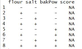
Now, we have eight different experiments (recipes) including all the possible combinations of the three factors at two levels.
When we have more than 2 factors, the combination of levels of different factors may affect the response. Therefore, to discover the main effects and the interactions, we should vary more than one level at a time, performing experiments in all the possible combinations.
The reason Why two-level factor experiments are widely used is that as the number of factor level increases, cost of doing the experiment increases. To study the variation under the same experimental conditions, replication needs to be done, making more than one trial per factor combination. The number of replications depends on several aspects (e.g budget).
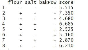
Once an experiment has been designed, we will proceed with its randomization.
pizzaDesign$ord <- sample(1:8, 8)
pizzaDesign[order(pizzaDesign$ord),]
Each time you repeat the command you get a different order due to randomization.
2^k factorial Designs
2k factorial designs are those whose number of factors to be studied are k, all of them with 2 levels. The number of experiments we need to carryout to obtain a complete replication is precisely the power(2 to the k). If we want n replications of the experiment, then the total number of experiments is n×2k.
ANOVA can be used to estimate the effect of each factor and interaction and assess which of these effects are significant.
Example contd.:- The experiment is carried out by preparing the pizzas at the factory following the package instructions, namely: “bake the pizza for 9 min in an oven at 180◦C.”
After a blind trial is conducted,the scores were given by the experts to each of the eight (2^3) recipes in each replication of the experiment.
ss.data.doe1 <- data.frame(repl = rep(1:2, each = 8), rbind(pizzaDesign[, -6], pizzaDesign[, -6]))
ss.data.doe1$score <- c(5.33, 6.99, 4.23, 6.61, 2.26, 5.75, 3.26, 6.24, 5.7, 7.71, 5.13, 6.76, 2.79, 4.57, 2.48, 6.18)
The average for each recipe can be calculated as below:
aggregate(score ~ flour + salt + bakPow, FUN = mean, data = ss.data.doe1)
The best recipe seems to be the one with a high level of flour and a low level of salt and baking powder. Fit a linear model and perform an ANOVA to find the significant effects.
doe.model1 <- lm(score ~ flour + salt + bakPow + flour * salt + flour * bakPow + salt * bakPow + flour * salt * bakPow, data = ss.data.doe1)


summary(doe.model1)
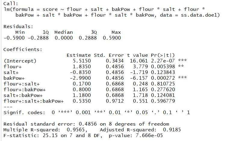
p-values show that the main effects of the ingredients flour and baking powder are significant, while the effect of the salt is not significant. Interactions among the ingredients are neither 2-way nor 3-way, making them insignificant. Thus, we can simplify the model, excluding the non significant effects. Thus, the new model with the significant effects is :
doe.model2 <- lm(score ~ flour + bakPow, data = ss.data.doe1)
summary(doe.model2)
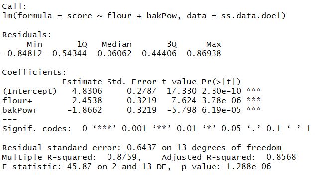
Therefore,the statistical model for our experiment is
score =4.8306 + 2.4538*Flour-1.8662*bakpow
Thus, the recipe with a high level of flour and low level of baking powder will be the best one, regardless of the level of salt (high or low). The estimated score for this recipe is
`4.8306 + 2.4538 × 1 + (−1.8662) × 0 = 7.284.`
predict function can be used to get the estimation for all the experiment conditions.
predict(doe.model2)

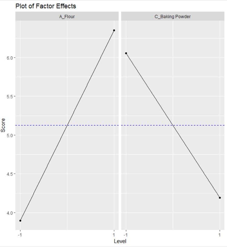
Visualize Effect Plot and Interaction plot
the ggplot2 package can be used to visualize the effect plot. The effect of flour is positive while the effect of baking powder is negative.
prinEf <- data.frame(Factor = rep(c("A_Flour", "C_Baking Powder"), each = 2), Level = rep(c(-1, 1), 2), Score = c(aggregate(score ~ flour, FUN = mean, data = ss.data.doe1)[,2], aggregate(score ~ bakPow, FUN = mean, data = ss.data.doe1)[,2]))
p <- ggplot(prinEf, aes(x = Level, y = Score)) + geom_point() + geom_line() +geom_hline(yintercept =mean(ss.data.doe1$score),linetype="dashed",
                                                                                        color = "blue")+scale_x_continuous(breaks = c(-1, 1)) + facet_grid(. ~ Factor)+ggtitle("Plot of Factor Effects")
print(p)
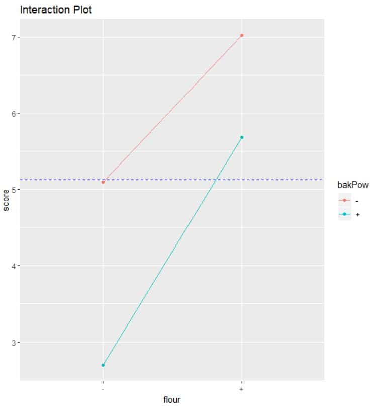
The interaction plot is as shown below.The lines don’t cross means that there is no interaction between the factors plotted.
intEf <- aggregate(score ~ flour + bakPow, FUN = mean, data = ss.data.doe1)
q <- ggplot(intEf, aes(x = flour, y = score, color = bakPow )) + geom_point() + geom_line(aes(group=bakPow)) +geom_hline(yintercept =mean(ss.data.doe1$score),linetype="dashed",
                                                                                                                        color = "blue")+ggtitle("Interaction Plot")
print(q)
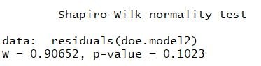
The normality of residual can be checked with Shapiro test. As the p-value is large, fail to reject the Null hypothesis of Normality of residuals.
shapiro.test(residuals(doe.model2))
This was the brief introduction to DOE in R.
In next part, we will go through Control Phase of Six Sigma DMAIC process. Please let me know your feedback in the comments section. Make sure to like & share it. Happy Learning!!