Understanding Titanic Dataset with H2O’s AutoML, DALEX, and lares library

If you have been studying or working with Machine Learning for at least a week, I am sure you have already played with the Titanic dataset! Today I bring some fun DALEX (Descriptive mAchine Learning EXplanations) functions to study the whole set’s response to the Survival feature and some individual explanation examples.

Before we start, I invite you all to install my personal library lares so you can follow step by step the following examples and use it to speed up your daily ML and Analytics tasks:

install.packages("lares")

A quick good model with h2o_automl

Let’s run the lares::h2o_automl function to generate a quick good model on the Titanic dataset. The lares library has this dataset already loaded, so with data(dft) you will load everything you need to reproduce these examples.

NOTE: when using the lares::h2o_automl function with our data frame as it is, with no ‘train_test’ parameter, it will automatically split 70/30 for our training and testing sets (use ‘split’ in the function if you want to change this relation).

library(lares)
library(dplyr)
data(dft) # Titanic dataset

results <- h2o_automl(dft, y = "Survived", 
                      ignore = c("Ticket","PassengerId","Cabind"), 
                      project = "Titanic Dataset",
                      max_models = 6, 
                      seed = 123)
2019-08-26 15:22:34 | Started process...
NOTE: The following variables contain missing observations: 'Age (19.87%)'. Consider setting the impute parameter.
NOTE: There are 6 non-numerical features. Consider using ohse() for One Hot Smart Encoding before automl if you want to custom your inputs.
Model type: Classifier
    tag   n     p   pcum
1 FALSE 549 61.62  61.62
2  TRUE 342 38.38 100.00
>>> Splitting datasets
train_size  test_size 
       623        268 
Algorithms excluded: 'StackedEnsemble', 'DeepLearning'
>>> Iterating until 6 models or 600 seconds...
Succesfully trained 6 models:
                                   model_id       auc   logloss
1              GBM_1_AutoML_20190826_102236 0.8850000 0.3862788
2              DRF_1_AutoML_20190826_102236 0.8808631 0.4039227
3          XGBoost_3_AutoML_20190826_102236 0.8720238 0.4233976
4          XGBoost_1_AutoML_20190826_102236 0.8610119 0.4318725
5          XGBoost_2_AutoML_20190826_102236 0.8588988 0.4396421
6 GLM_grid_1_AutoML_20190826_102236_model_1 0.8522619 0.4447343

[6 rows x 3 columns] 
Check results in H2O Flow's nice interface: http://localhost:54321/flow/index.html
Model selected: GBM_1_AutoML_20190826_102236
>>> Running predictions for Survived...
Target value: FALSE
>>> Generating plots...
Process duration: 15.59s
    AUC     ACC     PRC  TPR     TNR
1 0.885 0.85821 0.82979 0.78 0.90476
Warning messages:
1: In doTryCatch(return(expr), name, parentenv, handler) :
  Test/Validation dataset column 'Cabin' has levels not trained on: [A10, A19, A23, A5, B28, B3, B35, B73, B78, B79, B82 B84, B86, C103, C111, C87, C91, C92, D36, D45, D56, D6, E17, E31, E46, E68, E77, F2]
2: In doTryCatch(return(expr), name, parentenv, handler) :
  Test/Validation dataset column 'Embarked' has levels not trained on: []

Let’s quickly check our model’s performance with some plots:

plot(results$plots$dashboard)

Gives this plot:

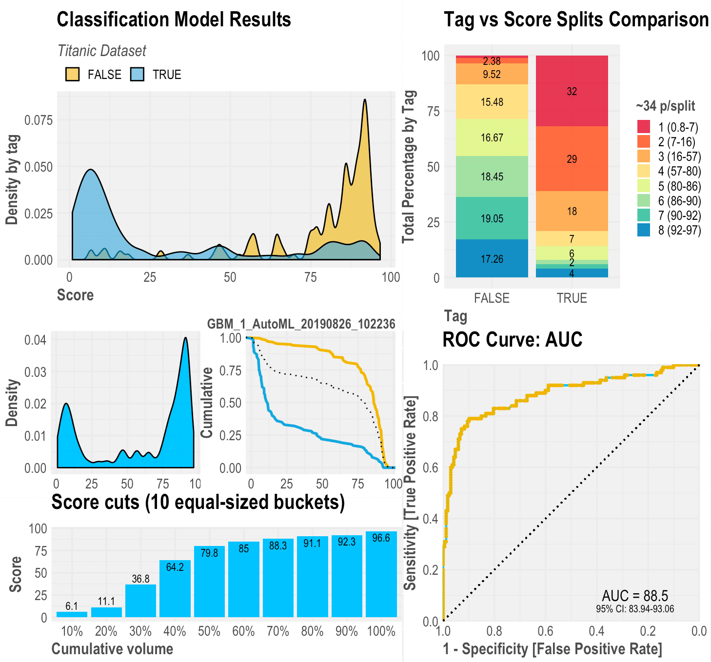
Basically, we got a very nice performing model, with an AUC of 88.5% which splits quite well the Titanic’s survivals. (Get much better models by increasing max_models parameter). Notice that from the top 25% scored-people, only 3% did not survive (the Captain? Sorry…) and 61% are true survivors.

Once we have this model, we can study which features did it chose as the most relevant and why. To understand this, there are probably more than a million ways, but today we are going to check the DALEX results.

The most important variables

Every dataset has relevant and irrelevant features. Sometimes it is our work as data scientist or analysts to detect which ones are these, how do they affect our independent variable and, most importantly, why. I happen to have the following function to help us see these results quickly:

results$plots$importance

Which will plot:

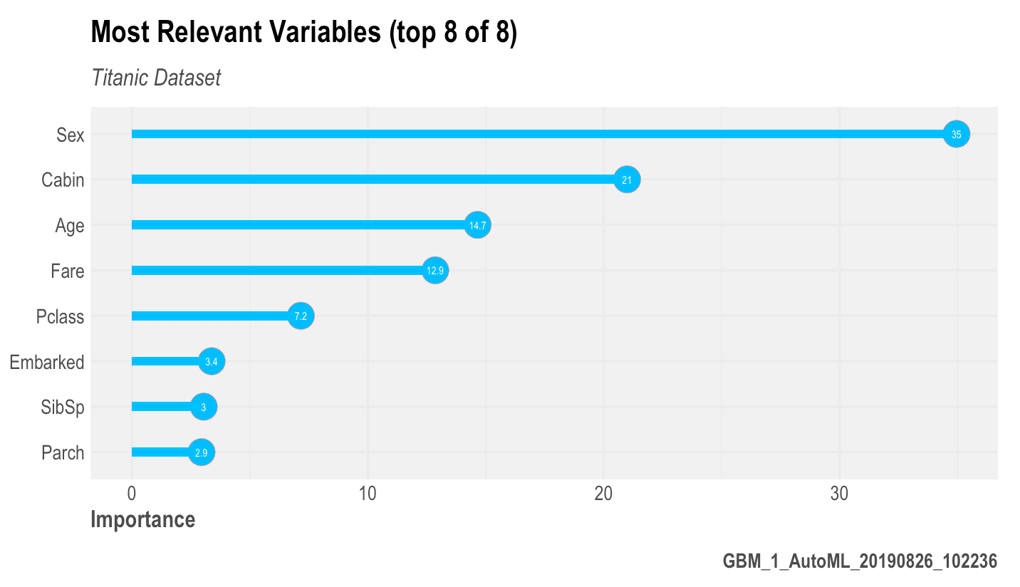
You can also plot something similar with the DALEX library but personally, I do like mine better! :$

Partial Dependency Plots (PDP)

Now that we know that Sex, Age, Fare, and Pclass are the most relevant features, we should check how the model detects the relationship between the target (Survival) and these features. Besides, these plots not only are incredibly powerful for communicating our insights to non-technical users but will also help us implement with more confidence our models (fewer black-boxes) into production.

To start plotting with DALEX (must be installed), we have to create an explainer. If you are using h2o or my functions above, this is all you need to do:

explainer <- dalex_explainer(
  df = filter(results$datasets$global, train_test == "train"), 
  model = results$model, 
  y = "Survived")
Preparation of a new explainer is initiated
  -> model label       :  GBM_1_AutoML_20190826_102236 
  -> data              :  623  rows  14  cols 
  -> target variable   :  623  values 
  -> predict function  :  h2o 
  -> predicted values  :  numerical, min =  0.01811329 , mean =  0.3886338 , max =  0.988011  
  -> residual function :  difference between y and yhat (default)
  -> residuals         :  numerical, min =  -0.8562805 , mean =  -0.0001908275 , max =  0.9191866  
A new explainer has been created!

So, let’s check our PDPs on our main features. Note that we will have different outputs regarding our variables’ class: if it’s a numerical value, then well have a Partial Dependency Plot (line-plot); if we have a categorical or factor variable, then we will get a Merging Path Plot (dendogram-plot).

sex <- dalex_variable(explainer, y = "Sex")
sex$plot

We get this plot:

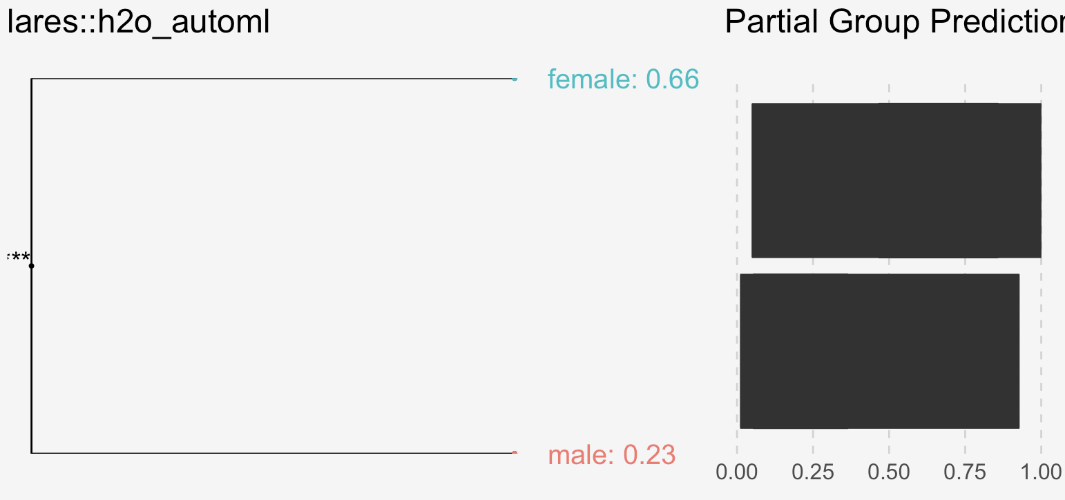
How chivalrous! Basically, if you were a man and survived, you were quite lucky (spoiler: and rich!).

age <- dalex_variable(explainer, "Age")
age$plot

We get this plot:

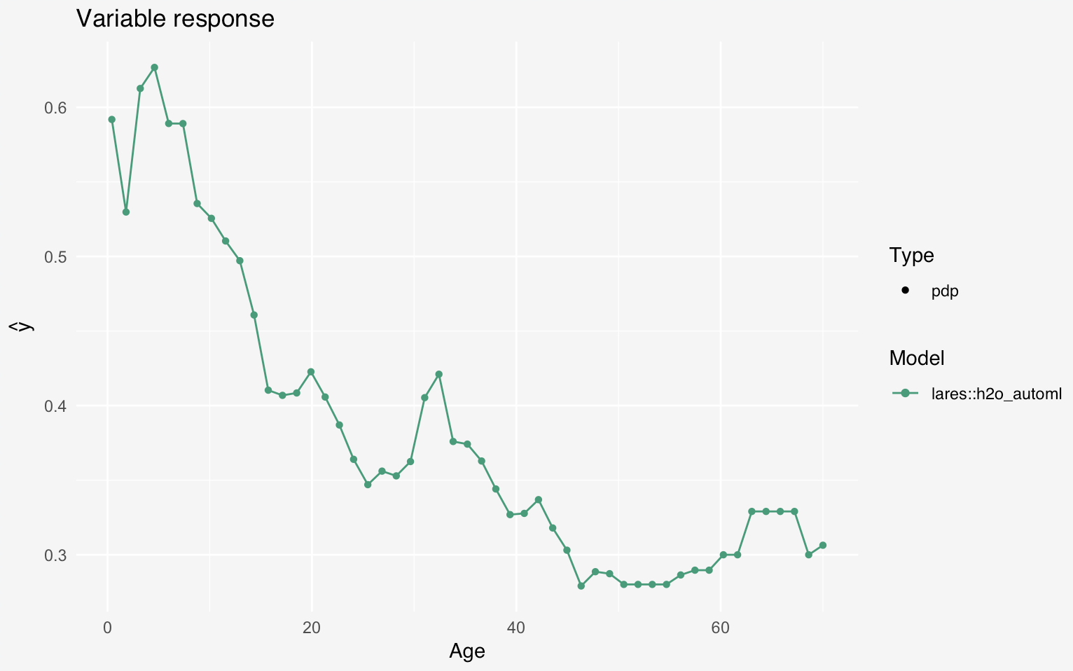
If you were a child, you shouldn’t even have to be scared when it all went ‘down’. Independently of your class, sex, and age, children were the ones who had a higher score, thus the highest probability of surviving. We get some picks around 33 years old and to hell with the elders.

fare <- dalex_variable(explainer, "Fare")
fare$plot

Another plot:

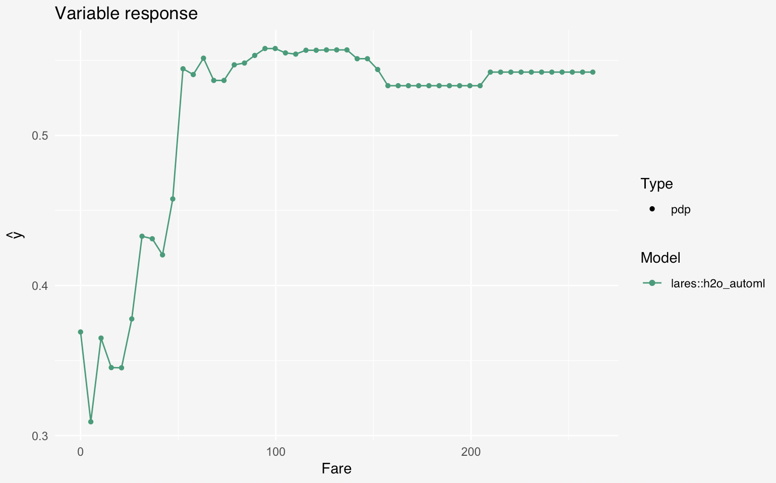
Basically, if you paid less than 50 bucks, you didn’t pay for the boats nor the lifesavers. So rude!

class <- dalex_variable(explainer, "Pclass", force_class = "factor")
class$plot

The plot:

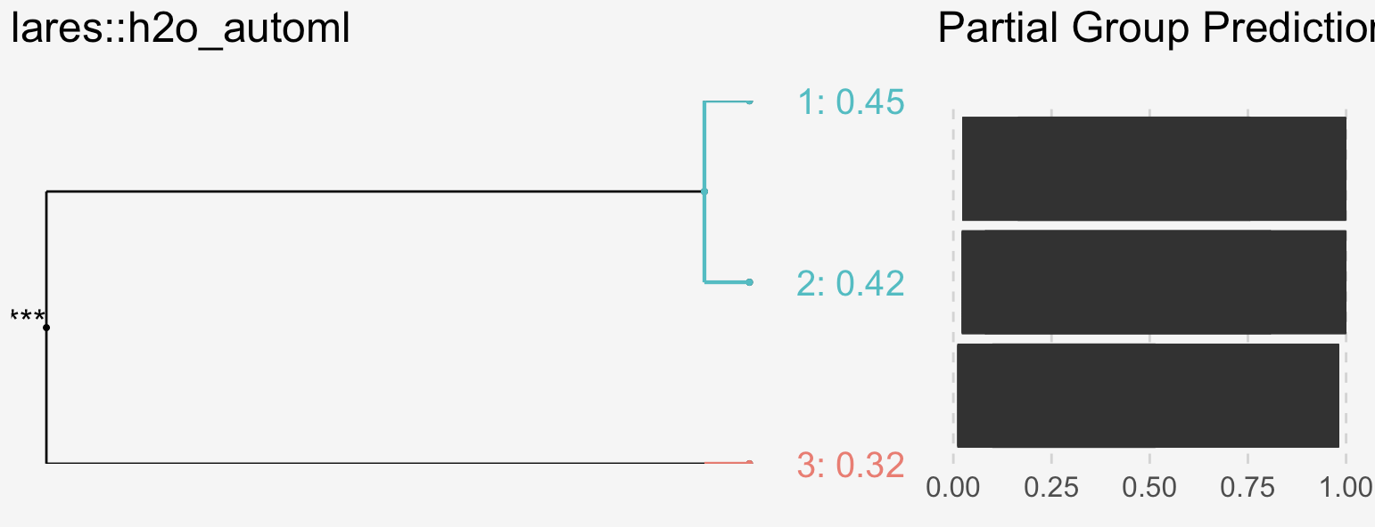
To emphasize once more on the economical situation vs survivals, we see how the 1st and 2nd classes were “luckier” than the 3rd class passengers.

With these plots (and with a little help from the movie to put us in perspective) we now can understand better the macro situation of Titanic’s survival. Now, let’s check some particular cases, as individuals, to go further into our analysis.

Individual Interpretation

The DALEX’s local interpretation functions are awesome! If you have used LIME before, in my taste, these are quite similar but better. Note than we can see that several predictors have zero contribution, while others have positive, and others negative contributions.

Before you start, let me tell you that each example we run lasts almost a minute to the plot… some patients when using this function!

Subject #1 (Randomly chose #23):

local23 <- dalex_local(explainer, observation = explainer$data[23,], plot = TRUE)

Gives this plot:

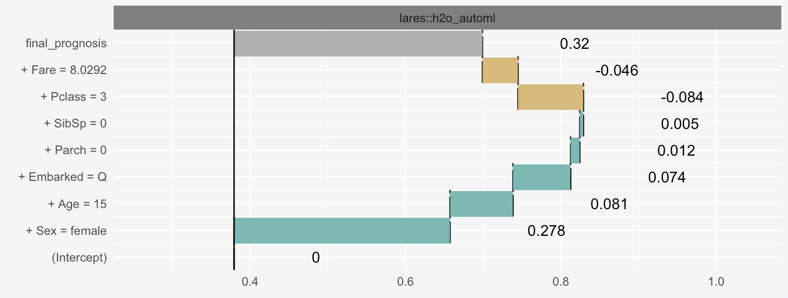
Here we can see a specific woman who scored pretty OK: 0.699 (can’t be seen in the image). The predicted value for this individual observation was positively and strongly influenced by the Sex = Female and Age = 15. Alternatively, the Pclass = 3 variable reduced this person’s probability of surviving.

Subject #2 (Worst score):

results$datasets$test[results$scores$score == min(results$scores$score),]
   tag Pclass  Sex Age SibSp Parch Fare Embarked
60   0      3 male  11     5     2 46.9        S

We have 1 person (out of 268) on our test set which scored 0.01. (Can’t help to mention that he really didn’t survive). Let’s study now this guy guy with our DALEX function:

local60 <- lares::dalex_local(explainer, observation = explainer$data[60,], plot = TRUE)

Gives this plot:

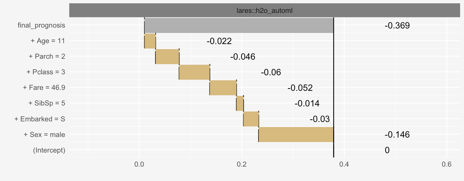
This poor boy sailed with a 3rd class ticket, having 11 years, traveling with 5 siblings and bot parents. The most important features were his Sex = male, and his low Fare/Pclass. Even though we noticed that children are more probable to have survived, this little man might be one of the exceptions because of (maybe) his amount of familiars onboard. If you think about it, the story behind it might be that he was in the ship with all his brothers and parents, which were 3rd class as well, and sinked with them instead of being save alone. Sad (but true) story.

Subject #3 (Best score):

If we repeat the prior example but with the highest score, we get 4 women, all 1st class, embarked through C Gates, and all 100% survivors. Let’s take a look at one:

local196 <- lares::dalex_local(explainer, row = 196)

The plot:

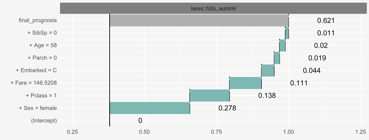
This handsome old lady, 58, traveled in first class with no family members, and payed a 147$ fare. Our model detects that this person had a very high probability of surviving, mainly because she payed a lot and is a woman!

Conclussions

• One way to understand a dataset is running a model and analyzing the Machine Learning’s intelligence behind.
• Studying the important variables on a macro view and some particular cases on a micro view will give us confidence and a global understanding.
• Partial dependence plots are a great way to extract insights from complex models. They can be very useful when showing our insights and results with other people.
• With DALEX we can stop showing our Machine Learning models to the world as plain black boxes.
• With the lares library we can automate and fasten our daily tasks for Analytics and Machine Learning jobs.

Hope this article was fun to read and something could be learnt! Don’t hesitate to comment beloew if you have any further question, comment or insight and I’ll be delighted to answer back as soon as possible. Please, keep in touch and feel free to contact me via Linkedin or email.