Most obesity numbers people quote come from asking: a phone survey asks for your height and weight, and BMI is computed from the answers. I wondered how far that drifts from what a scale and a stadiometer would say, and whether the error comes mostly from the weight people give or the height. The National Health and Nutrition Examination Survey can answer this directly, because it asks the same adults both questions at home and then measures them in a mobile exam center.
How do I compare self-reported and measured BMI in NHANES with R?
Join the questionnaire file (WHQ_L) to the exam file (BMX_L) by SEQN, turn the pound and inch answers into kg and cm, compute both BMIs for the same people, and estimate the two prevalences with survey::svymean() using the exam weight WTMEC2YR. The block below runs on its own and uses the August 2021 to August 2023 cycle, with R 4.6, haven 2.5.5 and survey 4.5.
library(tidyverse)
library(haven)
library(survey)

nhanes <- function(file) {
  path <- tempfile(fileext = ".xpt")
  url <- paste0("https://wwwn.cdc.gov/Nchs/Data/Nhanes/Public/2021/DataFiles/",
                file, ".xpt")
  download.file(url, path, mode = "wb", quiet = TRUE)
  read_xpt(path)
}

nh <- nhanes("DEMO_L") |>
  select(SEQN, RIAGENDR, RIDAGEYR, RIDEXPRG, WTMEC2YR, SDMVPSU, SDMVSTRA) |>
  left_join(nhanes("WHQ_L"), by = "SEQN") |>
  left_join(nhanes("BMX_L") |> select(SEQN, BMXWT, BMXHT), by = "SEQN")

nh <- nh |>
  mutate(
    # 7777 = refused, 9999 = don't know: not weights or heights
    across(c(WHD010, WHD020), \(x) if_else(x >= 7777, NA, x)),
    bmi_self = (WHD020 * 0.4536) / (WHD010 * 0.0254)^2,
    bmi_meas = BMXWT / (BMXHT / 100)^2,
    keep = RIDAGEYR >= 20 & coalesce(RIDEXPRG, 2) != 1 & WTMEC2YR > 0 &
      !is.na(bmi_self) & !is.na(bmi_meas)
  )

design <- svydesign(ids = ~SDMVPSU, strata = ~SDMVSTRA, weights = ~WTMEC2YR,
                    nest = TRUE, data = nh |> filter(WTMEC2YR > 0))
adults <- subset(design, keep)

obesity <- svymean(~I(bmi_self >= 30) + I(bmi_meas >= 30), adults)
obesity
##                           mean     SE
## I(bmi_self >= 30)FALSE 0.64605 0.0152
## I(bmi_self >= 30)TRUE  0.35395 0.0152
## I(bmi_meas >= 30)FALSE 0.60021 0.0179
## I(bmi_meas >= 30)TRUE  0.39979 0.0179
On 5,826 non-pregnant adults, BMI from their own answers puts 35.4% of American adults in the obese range (BMI 30 or more). Measured, it is 40.0%. That is a gap of 4.6 percentage points (95% CI 3.4 to 5.8), and it is not a wash of errors in both directions: 16% of adults who are obese by measurement, roughly one in six, would not be counted as obese from what they said.
Why does the average self-reported weight come out above 300 pounds?
Because NHANES stores "refused" as 7777 and "don’t know" as 9999 in the same numeric column as the real answers, so they have to be recoded to NA before any summary, which is what the across() line in the block above does. Without it, the mean weight adults report is absurd:
whq_raw <- nhanes("WHQ_L") |>
  semi_join(filter(nh, RIDAGEYR >= 20), by = "SEQN")

whq_raw |>
  summarise(coded_answers = sum(WHD020 >= 7777, na.rm = TRUE),
            raw_mean_lb   = mean(WHD020, na.rm = TRUE),
            clean_mean_lb = mean(if_else(WHD020 >= 7777, NA, WHD020), na.rm = TRUE))
## # A tibble: 1 × 3
##   coded_answers raw_mean_lb clean_mean_lb
##           <int>       <dbl>         <dbl>
## 1           109        308.          181.
Just 109 answers, 1.4% of the total, lift the mean from 181 to 308 pounds. The same convention (7, 9, 77, 99, 7777, 9999, scaled to the width of the field) runs through the whole survey, so check the codebook before summarising any NHANES variable. The answers that remain are rounded too: 64% of self-reported weights end in 0 or 5, where about 20% would by chance.
Height, not weight, is where the undercount comes from
On average adults overstate their height by 0.59 inches and understate their weight by 1.5 pounds. The weight error gets the attention, but swapping one self-reported value at a time into the measured BMI shows which one moves the obesity count more:
nh_swap <- update(adults,
  bmi_ht_only = BMXWT / (WHD010 * 0.0254)^2,
  bmi_wt_only = (WHD020 * 0.4536) / (BMXHT / 100)^2)

swap <- svymean(~I(bmi_meas >= 30) + I(bmi_ht_only >= 30) +
                  I(bmi_wt_only >= 30) + I(bmi_self >= 30), nh_swap)
tibble(bmi = c("measured", "self-reported height only",
               "self-reported weight only", "both self-reported"),
       obese = round(100 * coef(swap)[c(2, 4, 6, 8)], 1))
## # A tibble: 4 × 2
##   bmi                       obese
##   <chr>                     <dbl>
## 1 measured                   40
## 2 self-reported height only  37.1
## 3 self-reported weight only  38.4
## 4 both self-reported         35.4
The height answer alone takes 2.9 points off the obesity rate; the weight answer alone takes 1.6. Height enters BMI squared, so an inch is worth more than it looks, and the overstatement grows with age (0.34, 0.47, 1.00 inches across the three age bands below), which fits people going on reporting the height they had before they started losing it.
adults <- update(adults,
  age_band = cut(RIDAGEYR, c(19, 39, 59, 80), labels = c("20-39", "40-59", "60+")),
  sex = if_else(RIAGENDR == 1, "Men", "Women"),
  height_over = WHD010 - BMXHT / 2.54,
  weight_over = WHD020 - BMXWT / 0.4536)

groups <- svyby(~I(bmi_self >= 30) + I(bmi_meas >= 30) + height_over + weight_over,
                ~age_band + sex, adults, svymean) |>
  as_tibble(.name_repair = "minimal") |>
  select(age_band, sex, self = 4, measured = 6, height_over, weight_over)

dsp_colors <- c("#0066CC", "#E8862D", "#159A6C", "#7D5BD6",
                "#D64580", "#2AA9B8", "#C9A227")
dsp_theme <- theme_minimal(base_size = 13) +
  theme(plot.background    = element_rect(fill = "#ECECEF", color = NA),
        panel.background   = element_rect(fill = "#ECECEF", color = NA),
        panel.grid.minor   = element_blank(),
        panel.grid.major.x = element_blank(),
        panel.grid.major.y = element_line(color = "grey78"),
        axis.ticks         = element_blank(),
        plot.title         = element_text(face = "bold"),
        strip.text         = element_text(face = "bold"))

groups |>
  pivot_longer(c(self, measured), names_to = "source", values_to = "obese") |>
  ggplot(aes(age_band, obese, color = source)) +
  geom_line(aes(group = age_band), color = "grey55", linewidth = 1) +
  geom_point(size = 3.5) +
  facet_wrap(~sex) +
  scale_y_continuous(labels = scales::percent, limits = c(0.25, 0.5)) +
  scale_color_manual(values = dsp_colors, breaks = c("self", "measured"),
                     labels = c("Self-reported", "Measured")) +
  labs(title = "Obesity prevalence, US adults, NHANES 2021-2023",
       x = "Age", y = NULL, color = NULL) +
  dsp_theme +
  theme(legend.position = "top")
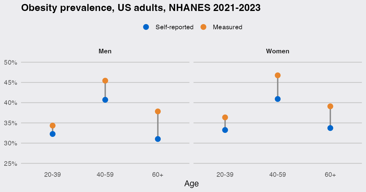
Men aged 60 and over make the point cleanly. They report weighing 0.9 pounds more than the scale says on average, so their weight answers push BMI up, yet their obesity rate still drops from 37.8% measured to 31.0% self-reported, because they overstate their height by 1.19 inches.
One caveat on the design: the questions are asked at home and the measurements are taken at a later exam visit, so some of the weight gap is real change in between. It is small here (the weighted median of self-reported minus measured weight is -0.6 pounds), and the height gap cannot be explained that way at all: adults do not lose an inch in a few weeks.
If you work with obesity figures built from answers rather than measurements, treat them as a floor. In this cycle the floor sits about 5 points below the measured rate, and most of the distance is inches, not pounds.


