
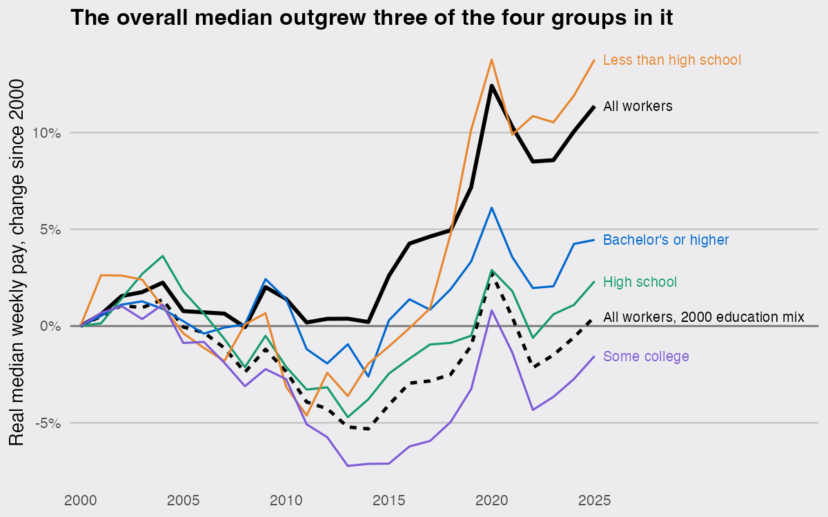
The median US full-time worker aged 25 and over earned $1,268 a week in 2025, 11.4% more than in 2000 after inflation. I wanted to know who got that raise, so I split the same workers by education, and the raise mostly disappears. Real median pay rose 2.3% for high school graduates and 4.5% for people with a bachelor’s degree or more, and it fell 1.6% for people with some college. Only the smallest group, workers without a high school diploma (5.4% of the total in 2025), beat the overall figure.
The overall median can outrun almost every group because the groups changed size. Workers with a bachelor’s degree or more went from 31.1% of full-time workers in 2000 to 47.3% in 2025, and they are the best-paid group. Rebuild the 2025 pay distribution with 2000’s education mix and the median comes out at $1,141 a week, only 0.5% above 2000 in real terms: about 96% of the rise in the median comes from who is working, not from what any group is paid.
The BLS earnings data
The numbers are the Bureau of Labor Statistics’ usual weekly earnings of full-time wage and salary workers aged 25 and over, from the Current Population Survey, as annual averages. For each of four education groups BLS publishes the number of workers and five points of the pay distribution: the 10th, 25th, 50th, 75th and 90th percentiles. The block below pulls all 30 series plus the consumer price index (CPIAUCNS) from FRED and puts every year in 2025 dollars. It runs on its own with dplyr 1.2.1, readr 2.2.0 and httr2 1.3.0 on R 4.6.1.
library(tidyverse)
library(httr2)   # as of October 2026, FRED refuses R's default user agent

fred <- function(id) {
  request("https://fred.stlouisfed.org/graph/fredgraph.csv") |>
    req_url_query(id = id) |>
    req_perform() |>
    resp_body_string() |>
    I() |>
    read_csv(show_col_types = FALSE) |>
    set_names(c("date", "value")) |>
    mutate(year = year(date), .keep = "unused")
}

# BLS series IDs: workers (thousands) and weekly earnings percentiles
series <- tribble(
  ~group,                 ~n,              ~p10,            ~p25,            ~p50,            ~p75,            ~p90,
  "All",                  "LEU0252887600", "LEU0252916000", "LEU0252916100", "LEU0252887700", "LEU0252916200", "LEU0252916300",
  "Less than high school","LEU0252916400", "LEU0252916500", "LEU0252916600", "LEU0252916700", "LEU0252916800", "LEU0252916900",
  "High school",          "LEU0252917000", "LEU0252917100", "LEU0252917200", "LEU0252917300", "LEU0252917400", "LEU0252917500",
  "Some college",         "LEU0254929100", "LEU0254929200", "LEU0254929300", "LEU0254929400", "LEU0254929500", "LEU0254929600",
  "Bachelor's or higher", "LEU0252918200", "LEU0252918300", "LEU0252918400", "LEU0252918500", "LEU0252918600", "LEU0252918700"
)

# October 2025 was never collected (federal shutdown); BLS's annual average uses the other 11 months
cpi <- fred("CPIAUCNS") |>
  summarise(cpi = mean(value, na.rm = TRUE), .by = year)
cpi_2025 <- cpi$cpi[cpi$year == 2025]

pay <- series |>
  pivot_longer(-group, names_to = "stat", values_to = "id") |>
  mutate(data = map(id, \(x) fred(paste0(x, "A")))) |>   # "A": the annual-average series
  unnest(data) |>
  select(-id) |>
  pivot_wider(names_from = stat, values_from = value) |>
  filter(between(year, 2000, 2025)) |>
  left_join(cpi, by = "year") |>
  mutate(across(p10:p90, \(x) x * cpi_2025 / cpi))       # 2025 dollars
The na.rm = TRUE on the CPI matters for 2025 only: without it the 2025 average is NA, and so is every converted figure. With it the average is 321.943, the figure BLS published.
How do I combine group medians into an overall median in R?
You cannot average them, not even weighted by group size: rebuild each group’s pay distribution from its published percentiles, mix the distributions in proportion to the number of workers, and find where the mix crosses one half. A median depends on the whole shape of each group’s distribution, which a weighted mean of four medians ignores. For 2025 that shortcut gives $1,353, 6.7% above the $1,268 BLS published. The block below runs on its own with the 2025 figures typed in:
library(purrr)

# 2025 annual averages, full-time wage and salary workers aged 25+ (BLS, CPS)
groups_2025 <- tibble::tribble(
  ~group,                  ~n,    ~p10, ~p25, ~p50, ~p75, ~p90,
  "Less than high school",  6012,  493,  613,  770, 1002, 1381,
  "High school",           26126,  586,  729,  966, 1374, 1910,
  "Some college",          26223,  632,  806, 1097, 1568, 2227,
  "Bachelor's or higher",  52484,  835, 1166, 1740, 2586, 3848
)

# A group's CDF: a monotone spline through its five percentiles, drawn on a
# log-pay / normal-score scale, where earnings are close to a straight line
group_cdf <- function(p10, p25, p50, p75, p90) {
  s <- splinefun(log(c(p10, p25, p50, p75, p90)), qnorm(c(.10, .25, .50, .75, .90)),
                 method = "monoH.FC")
  \(v) pnorm(s(log(v)))
}

# The pooled CDF is the size-weighted mix of the group CDFs
pooled_quantile <- function(cdfs, n, p = 0.5) {
  w <- n / sum(n)
  uniroot(\(v) sum(w * map_dbl(cdfs, \(F) F(v))) - p, c(1, 1e5))$root
}

cdfs <- pmap(groups_2025[c("p10", "p25", "p50", "p75", "p90")], group_cdf)
pooled_quantile(cdfs, groups_2025$n)              # BLS published 1,268
## [1] 1271.727
weighted.mean(groups_2025$p50, groups_2025$n)     # the shortcut
## [1] 1352.842
The rebuilt median is $1,272. Run for every year from 2000 to 2025 against the published "All" figure, the method is never more than 0.7% off. The spline needs the monoH.FC method, which keeps it increasing, so the CDF can never bend backwards between two percentiles.
Holding the 2000 workforce fixed
The same two functions answer the counterfactual. Give each year’s group distributions the 2000 group sizes instead of their own:
by_group <- pay |>
  filter(group != "All") |>
  mutate(cdf = pmap(list(p10, p25, p50, p75, p90), group_cdf))

mix_2000 <- by_group |> filter(year == 2000) |> select(group, n_2000 = n)

trend <- by_group |>
  left_join(mix_2000, by = "group") |>
  summarise(actual_mix = pooled_quantile(cdf, n),
            mix_2000   = pooled_quantile(cdf, n_2000),
            .by = year)

max_err <- trend |>
  left_join(filter(pay, group == "All"), by = "year") |>
  summarise(max(abs(actual_mix / p50 - 1))) |>
  pull()
With the 2000 mix the 2025 median is $1,141, against $1,272 with the real one and $1,135 (in 2025 dollars) in 2000. Of the $136 a week the median gained, $131 is the shift in education. In the chart the dashed line sits below zero in 18 of the 25 years after 2000, and the gap between it and the solid line, the education effect, widens in 23 of them. The jump every line makes in 2020 is the same effect inside each group: lower-paid workers lost their jobs, so the median of those still at work went up.
Two limits on reading this. The counterfactual keeps each group’s pay as it was, while in a world with fewer graduates a degree would probably pay more. And "education" here carries whatever moved with it, such as age and the growing share of advanced degrees inside the top group. The finding is narrower than "nobody got a raise": the typical full-time worker in 2025 earns more mostly because more of them hold degrees, while the median within each group, except the smallest one, moved less than 5% in 25 years.
