
In the 12 months to May 2026, 66,478 people died of drug overdoses in the United States, by CDC’s provisional count adjusted for records still pending. That is 41% below the peak of 112,418 in the 12 months to August 2023, 7% below 2019, and the lowest 12-month total since the period ending January 2017. I wondered whether the whole country is back to where it was before the surge, or whether the national number is averaging something away.
It is averaging away a regional split. The Northeast is 32% below its 2019 level and the Midwest 27% below, while the West is 46% above it. Per resident, the West has gone from the lowest overdose death rate of the four Census regions in 2019, 18.1 per 100,000, to the highest in the latest 12 months, 26.0, while the Northeast fell from the highest, 28.2, to 18.6.
How do I compare trends across states of very different sizes in R?
Divide each state’s series by its own value in a reference period, inside a grouped mutate(), so every state becomes a ratio to the same moment and 1.5 means the same thing in Wyoming as in California. The data is the National Center for Health Statistics’ VSRR Provisional Drug Overdose Death Counts, a public-domain CSV on data.cdc.gov that needs no key, here with deaths through May 2026. This block runs on its own (R 4.6.1, dplyr 1.2.1):
library(tidyverse)

vsrr <- read_csv("https://data.cdc.gov/api/views/xkb8-kh2a/rows.csv?accessType=DOWNLOAD",
                 show_col_types = FALSE)

od <- vsrr |>
  filter(Indicator == "Number of Drug Overdose Deaths", State != "PR") |>
  mutate(date   = ymd(paste(Year, Month, 1)),
         deaths = coalesce(`Predicted Value`, `Data Value`),
         state  = if_else(State == "YC", "NY", State)) |>  # NY excludes New York City
  summarise(deaths = sum(deaths), reported = sum(`Data Value`), .by = c(state, date))

latest <- max(od$date)

indexed <- od |>
  filter(state != "US") |>
  mutate(vs_2019 = deaths / deaths[date == ymd("2019-12-01")],
         vs_peak = deaths / max(deaths), .by = state)

indexed |>
  filter(date == latest) |>
  summarise(states = n(), below_peak = sum(vs_peak < 1), above_2019 = sum(vs_2019 > 1))
## # A tibble: 1 × 3
##   states below_peak above_2019
##    <int>      <int>      <int>
## 1     51         50         26
Three things in this file change the numbers before any chart does. Every row is a total for the 12 months ending in that month, not a monthly count: summing the twelve 2025 rows for the US gives 892,682 deaths, while the 2025 total is the December row, 70,735. Data Value is the count reported so far and Predicted Value is CDC’s estimate after adjusting for death records still pending investigation; I use the predicted value throughout (the last section shows why). And the NY row excludes New York City, which has its own row, YC. Alone, NY is 21% below 2019 and looks like one of the recovered states; New York City is 21% above; the state as a whole is 4% below. Puerto Rico is in the file but not in the US total, so I leave it out.
Down from the peak is not back to 2019
The reference period decides the story. Against each state’s own peak, 50 of the 51 states (counting DC) are down; the exception is New Mexico, whose latest 12 months are its worst yet. Against 2019, 26 of the 51 are still above, including every one of the 13 Western states (Idaho only just). Grouping the states into Census regions shows where the split runs. I set the house plot theme once here and reuse it:
dsp_colors <- c("#0066CC", "#E8862D", "#159A6C", "#7D5BD6",
                "#D64580", "#2AA9B8", "#C9A227")
dsp_theme <- theme_minimal(base_size = 13) +
  theme(plot.background    = element_rect(fill = "#ECECEF", color = NA),
        panel.background   = element_rect(fill = "#ECECEF", color = NA),
        panel.grid.minor   = element_blank(),
        panel.grid.major.x = element_blank(),
        panel.grid.major.y = element_line(color = "grey78"),
        axis.ticks         = element_blank(),
        plot.title         = element_text(face = "bold"),
        strip.text         = element_text(face = "bold"))

regions <- tibble(state  = c(state.abb, "DC"),
                  region = c(as.character(state.region), "South")) |>
  mutate(region = if_else(region == "North Central", "Midwest", region))

by_region <- od |>
  inner_join(regions, by = "state") |>
  summarise(deaths = sum(deaths), .by = c(region, date)) |>
  mutate(vs_2019 = deaths / deaths[date == ymd("2019-12-01")], .by = region)

ggplot(by_region, aes(date, vs_2019, color = region)) +
  geom_hline(yintercept = 1, linetype = "dashed", color = "grey40") +
  geom_line(linewidth = 1.1) +
  scale_color_manual(values = dsp_colors) +
  scale_y_continuous(labels = scales::label_percent(), breaks = seq(0.5, 2, 0.25)) +
  labs(x = NULL, y = "12-month overdose deaths, % of 2019", color = NULL,
       title = "Every region but the West is back below 2019") +
  dsp_theme +
  theme(legend.position = "top")
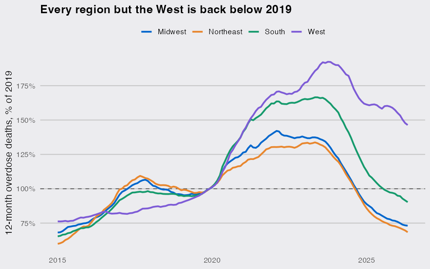
The West’s surge came later and has receded less. Its 12-month count peaked in October 2023 and is down 24% since, against falls of 46% to 49% in the other three regions. State by state, the dot is the latest 12 months and the open circle is the peak, both relative to 2019:
snap <- indexed |>
  summarise(peak = max(vs_2019), now = vs_2019[date == latest], .by = state) |>
  inner_join(regions, by = "state") |>
  mutate(name = if_else(state == "DC", "District of Columbia", state.name[match(state, state.abb)]),
         name = fct_reorder(name, now))

ggplot(snap, aes(y = name)) +
  geom_vline(xintercept = 1, linetype = "dashed", color = "grey40") +
  geom_segment(aes(x = now, xend = peak, yend = name), color = "grey60") +
  geom_point(aes(x = peak), shape = 21, fill = "#ECECEF", color = "grey40", size = 2) +
  geom_point(aes(x = now, color = region), size = 2.8) +
  scale_x_log10(breaks = c(0.5, 0.75, 1, 1.5, 2, 3),
                labels = c("0.5x", "0.75x", "1x", "1.5x", "2x", "3x")) +
  scale_color_manual(values = dsp_colors) +
  labs(x = "12-month overdose deaths relative to 2019", y = NULL, color = NULL,
       title = "All but one state is below its peak,\nhalf are still above 2019") +
  dsp_theme +
  theme(legend.position = "top")
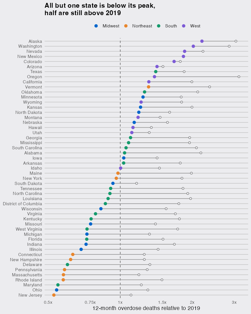
Alaska (2.2 times its 2019 count) and Washington (2.0 times) are about double; New Jersey and Ohio are about half, 47% and 46% below.
The West went from the lowest death rate to the highest
Counts can mislead when state populations grow at different speeds, so I divided by the Census Bureau’s population estimates (Vintage 2019 for 2019, Vintage 2025 for the latest 12 months). CDC counts deaths in the state where they occur, so this is a rate per resident only approximately:
pop <- bind_rows(
  read_csv("https://www2.census.gov/programs-surveys/popest/datasets/2010-2019/national/totals/nst-est2019-alldata.csv",
           show_col_types = FALSE) |> transmute(SUMLEV, NAME, year = 2019, pop = POPESTIMATE2019),
  read_csv("https://www2.census.gov/programs-surveys/popest/datasets/2020-2025/state/totals/NST-EST2025-ALLDATA.csv",
           show_col_types = FALSE) |> transmute(SUMLEV, NAME, year = 2025, pop = POPESTIMATE2025)
) |>
  filter(SUMLEV == "040") |>
  mutate(state = c(state.abb, "DC")[match(NAME, c(state.name, "District of Columbia"))])

rates <- od |>
  filter(date %in% c(ymd("2019-12-01"), latest)) |>
  mutate(year = if_else(date == latest, 2025, 2019)) |>
  inner_join(pop, by = c("state", "year")) |>
  inner_join(regions, by = "state") |>
  summarise(per_100k = sum(deaths) / sum(pop) * 1e5, .by = c(region, year)) |>
  pivot_wider(names_from = year, values_from = per_100k) |>
  rename(in_2019 = `2019`, latest = `2025`) |>
  arrange(desc(latest))
rates
## # A tibble: 4 × 3
##   region    in_2019 latest
##   <chr>       <dbl>  <dbl>
## 1 West         18.1   26.0
## 2 Northeast    28.2   18.6
## 3 South        20.8   17.6
## 4 Midwest      23.1   16.6
Per resident, the West is 43% above 2019, close to the 46% from raw counts, so population growth does not explain it. The likelier explanation is timing. In the 2019 records, synthetic opioids other than methadone (in practice, mostly illicit fentanyl) were involved in 27% of overdose deaths in the 11 Western states that report drug detail, against 75% in the Northeast:
fent <- vsrr |>
  filter(Year == 2019, Month == "December", State != "PR",
         Indicator %in% c("Number of Drug Overdose Deaths",
                          "Synthetic opioids, excl. methadone (T40.4)")) |>
  mutate(state = if_else(State == "YC", "NY", State)) |>
  summarise(n = sum(`Predicted Value`), .by = c(state, Indicator)) |>
  pivot_wider(names_from = Indicator, values_from = n) |>
  rename(all = "Number of Drug Overdose Deaths",
         fentanyl = "Synthetic opioids, excl. methadone (T40.4)") |>
  filter(!is.na(fentanyl)) |>  # drug detail is suppressed where it is incomplete
  inner_join(regions, by = "state") |>
  summarise(states = n(), share = sum(fentanyl) / sum(all), .by = region)
fent
## # A tibble: 4 × 3
##   region    states share
##   <chr>      <int> <dbl>
## 1 West          11 0.267
## 2 Northeast      8 0.752
## 3 South         14 0.510
## 4 Midwest        8 0.607
The East’s 2019 baseline was already a fentanyl year. The West’s was not, so the same national decline leaves the West far above where it started.
Recent months are still coming in
Oregon’s reported count falls from 1,406 in the 12 months to August 2025 to 629 in the 12 months to May 2026, a 55% drop in nine months. Part of it is records that are not in yet: 2.4% of Oregon’s recent death records are still pending investigation (0.24% nationally), and CDC’s predicted value for the same period is 848, about 35% higher. Plot Data Value and Oregon shows the steepest fall from its peak of any state (67%); with the predicted value the fall is 56%, and the steepest belongs to Rhode Island (61%). CDC’s technical notes warn that where more than 1% of records are pending, provisional counts can understate the final count by as much as 30%, and that the adjustment may not fully catch unusually long delays, so the predicted figure for Oregon may still be low.
The national total is now pulled down mostly by the large Eastern states where fentanyl arrived first and is receding first. A state chart indexed to a pre-surge year, with New York City added back into New York and the predicted column used for recent months, is the version that shows where overdose deaths are still high.
