
I was reading R’s own help pages back to back when I noticed that its defaults contradict each other. t.test() compares two groups without assuming their variances are equal: the var.equal argument defaults to FALSE, so the plain call is Welch’s t-test. Add a third group, reach for aov(), and the assumption quietly comes back, because a linear model has exactly one residual variance to hand out. Same data, same question, and the default answer changed on the way from two groups to three.
R already ships the version that keeps its promise. It is one function call, and it is not aov().
How do I run a one-way ANOVA in R without assuming equal variances?
Use oneway.test(). Its var.equal argument defaults to FALSE, so the plain call is already the Welch ANOVA, no extra argument and no extra package. Everything below runs on base R plus palmerpenguins, on R 4.6.1.
library(palmerpenguins)
library(dplyr)

penguins_ok <- penguins |> filter(!is.na(body_mass_g))

oneway.test(body_mass_g ~ island, data = penguins_ok)
##
## 	One-way analysis of means (not assuming equal variances)
##
## data:  body_mass_g and island
## F = 106.97, num df = 2.00, denom df = 150.41, p-value < 2.2e-16
Compare that with the pooled-variance version everyone writes:
summary(aov(body_mass_g ~ island, data = penguins_ok))
##              Df    Sum Sq  Mean Sq F value Pr(>F)
## island        2  86314512 43157256     110 <2e-16 ***
## Residuals   339 132993186   392310
## ---
## Signif. codes:  0 '***' 0.001 '**' 0.01 '*' 0.05 '.' 0.1 ' ' 1
Both say the islands differ, but look at the denominator degrees of freedom: aov() spends 339, Welch spends 150.4. That gap is the price of admitting the groups have different spreads, and here they clearly do.
penguins_ok |>
  group_by(island) |>
  summarise(n = n(), mean = mean(body_mass_g), sd = sd(body_mass_g))
## # A tibble: 3 × 4
##   island        n  mean    sd
##   <fct>     <int> <dbl> <dbl>
## 1 Biscoe      167 4716.  783.
## 2 Dream       124 3713.  417.
## 3 Torgersen    51 3706.  445.
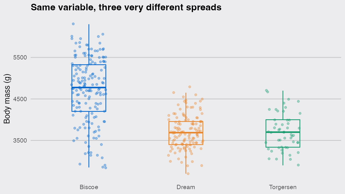
Biscoe hosts both Adelie and Gentoo penguins and Gentoo are much heavier, so its spread (783 g) is nearly twice Dream’s (417 g). Torgersen has only Adelie penguins and only 51 of them. Unequal group sizes and unequal spreads in the same table is exactly the situation the pooled test handles badly.
library(ggplot2)

dsp_colors <- c("#0066CC", "#E8862D", "#159A6C", "#7D5BD6",
                "#D64580", "#2AA9B8", "#C9A227")
dsp_theme <- theme_minimal(base_size = 13) +
  theme(plot.background    = element_rect(fill = "#ECECEF", color = NA),
        panel.background   = element_rect(fill = "#ECECEF", color = NA),
        panel.grid.minor   = element_blank(),
        panel.grid.major.x = element_blank(),
        panel.grid.major.y = element_line(color = "grey78"),
        axis.ticks         = element_blank(),
        plot.title         = element_text(face = "bold"),
        strip.text         = element_text(face = "bold"))

ggplot(penguins_ok, aes(island, body_mass_g, color = island)) +
  geom_jitter(width = 0.18, alpha = 0.35, size = 1.4) +
  geom_boxplot(width = 0.35, fill = NA, outlier.shape = NA, linewidth = 0.6) +
  scale_color_manual(values = dsp_colors, guide = "none") +
  labs(title = "Same variable, three very different spreads",
       x = NULL, y = "Body mass (g)") +
  dsp_theme
Why does t.test() give a different p-value than aov() on the same two groups?
Because they make different assumptions by default. t.test() runs Welch unless you pass var.equal = TRUE; aov() and summary(lm()) always pool. On two groups the pooled t-test and the one-way ANOVA are the same test, so if t.test() and aov() disagree on your data, the disagreement is the variance assumption and nothing else.
two <- penguins_ok |> filter(island %in% c("Biscoe", "Torgersen"))

c(welch  = t.test(body_mass_g ~ island, data = two)$parameter,
  pooled = t.test(body_mass_g ~ island, data = two, var.equal = TRUE)$parameter)
##  welch.df pooled.df
##    149.03    216.00
149.03 degrees of freedom against 216, from the same 218 penguins. On these two islands the body mass difference is so large that both tests land below 2e-16 and you would never see the disagreement. It shows up where decisions actually get made, near the 5% line, and how big it gets depends on the way the group sizes and the spreads line up.
What pooling the variance actually costs
The honest way to see it is to erase the effect and count false alarms. I kept the real design, the observed group sizes and standard deviations, generated data with all three means identical, and asked how often each test rejects at the 5% level. Then I flipped which group carries the big spread, and finally equalised the group sizes.
library(purrr)
library(tidyr)

sim_p <- function(n, sd, mu = rep(0, length(n))) {
  g <- factor(rep(seq_along(n), n))
  y <- rnorm(sum(n), mean = rep(mu, n), sd = rep(sd, n))
  c(classic = summary(aov(y ~ g))[[1]][["Pr(>F)"]][1],
    welch   = oneway.test(y ~ g)$p.value)
}

designs <- tibble(
  design = c("As observed", "Big spread on small group", "Equal group sizes"),
  n      = list(c(167, 124, 51), c(167, 124, 51), c(114, 114, 114)),
  sd     = list(c(783, 417, 445), c(445, 417, 783), c(445, 417, 783))
)

set.seed(1)
reps <- 20000

false_positives <- designs |>
  mutate(p = map2(n, sd, \(nn, ss) {
    runs <- map(seq_len(reps), \(i) sim_p(nn, ss))
    tibble(classic = map_dbl(runs, "classic"), welch = map_dbl(runs, "welch"))
  })) |>
  select(design, p) |>
  unnest(p) |>
  pivot_longer(c(classic, welch), names_to = "test", values_to = "p") |>
  group_by(design, test) |>
  summarise(rate = mean(p < 0.05), .groups = "drop")

false_positives
## # A tibble: 6 × 3
##   design                    test      rate
##   <chr>                     <chr>    <dbl>
## 1 As observed               classic 0.0242
## 2 As observed               welch   0.0492
## 3 Big spread on small group classic 0.131
## 4 Big spread on small group welch   0.0489
## 5 Equal group sizes         classic 0.0588
## 6 Equal group sizes         welch   0.0515
The pooled test is not merely approximate here, it is wrong in a direction that depends on the design. With the spread the penguins actually have, where the largest group is also the most variable, aov() rejects a true null only 2.4% of the time instead of 5%: conservative, and quietly short on power. Move the big spread onto the smallest group and the same test rejects 13.1% of the time, more than double its nominal rate. Welch stays at 4.9% and 4.9% across both.
false_positives |>
  mutate(test = if_else(test == "classic", "aov()", "oneway.test()")) |>
  ggplot(aes(design, rate, fill = test)) +
  geom_col(position = position_dodge(width = 0.7), width = 0.6) +
  geom_hline(yintercept = 0.05, linetype = "dashed", color = "grey35") +
  geom_text(aes(label = sprintf("%.1f%%", 100 * rate)),
            position = position_dodge(width = 0.7), vjust = -0.6, size = 3.6) +
  scale_fill_manual(values = dsp_colors, name = NULL) +
  scale_y_continuous(labels = scales::percent, limits = c(0, 0.15)) +
  labs(title = "False positives at a nominal 5%, 20,000 null datasets each",
       x = NULL, y = NULL) +
  dsp_theme
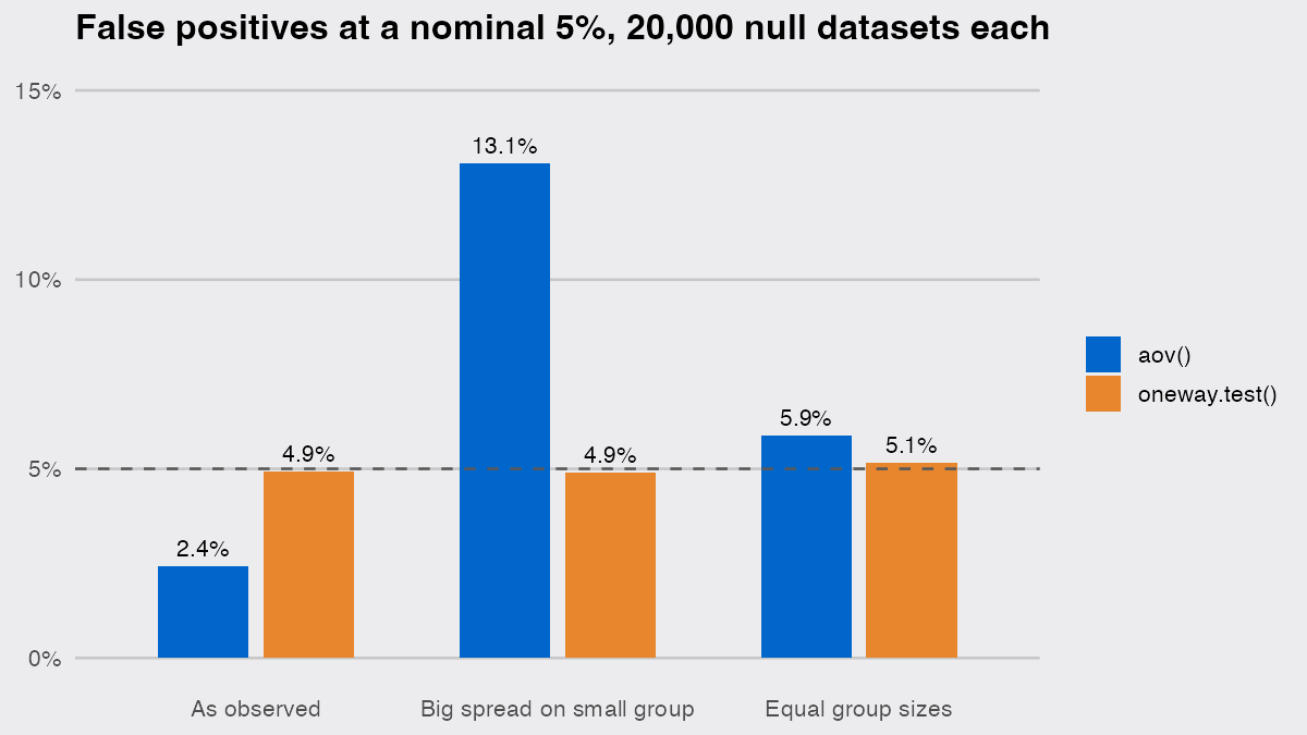
The third design is the reason this is not a crisis in every textbook example. Give the three groups the same size and the same badly unequal spreads, and aov() lands at 5.9%, close enough to 5% that nobody notices. Balanced designs really are robust to unequal variance. Unbalanced ones are not, and most real data is unbalanced.
The reverse cost is small. When the variances genuinely are equal, Welch gives up very little power:
set.seed(2)
pw <- map(seq_len(10000), \(i) sim_p(rep(20, 3), rep(1, 3), mu = c(0, 0.8, 0.8)))
power <- c(classic = mean(map_dbl(pw, "classic") < 0.05),
           welch   = mean(map_dbl(pw, "welch") < 0.05))
power
## classic   welch
##  0.7263  0.7109
On three equal groups of 20 with equal variances and a true difference of 0.8 standard deviations, aov() detects it 72.6% of the time and oneway.test() 71.1% of the time, a gap of about one and a half percentage points. That is what the insurance costs.
Do not let the follow-up tests smuggle the assumption back
TukeyHSD() only accepts an aov object and builds every interval from the pooled standard error, so running Welch for the omnibus test and Tukey for the pairwise comparisons puts the assumption straight back in. The base R follow-up that matches Welch is pairwise.t.test() with pool.sd = FALSE, which runs a Welch t-test per pair and adjusts the p-values.
pairwise.t.test(penguins_ok$body_mass_g, penguins_ok$island,
                pool.sd = FALSE, p.adjust.method = "holm")
##
## 	Pairwise comparisons using t tests with non-pooled SD
##
## data:  penguins_ok$body_mass_g and penguins_ok$island
##
##           Biscoe Dream
## Dream     <2e-16 -
## Torgersen <2e-16 0.93
##
## P value adjustment method: holm
What you lose by switching is real but narrow: oneway.test() returns a htest, not a model, so there are no residuals to plot, no coefficients, no TukeyHSD(), and nothing to pass to anova() for model comparison. If you need the fitted model, keep lm() and get heteroscedasticity-consistent tests from it instead, with car::Anova(fit, white.adjust = TRUE).
For the common case, though, the rule is short. If your groups are unbalanced and their spreads differ, aov() is answering a slightly different question than the one you asked, and oneway.test() is the same length to type.
