
New York City grades its restaurants from the points an inspector hands out: 0 to 13 points earns an A, 14 to 27 a B, 28 or more a C, and the letter goes in the window. I wanted to see what the scores themselves look like, and the answer turned out to depend almost entirely on how the histogram is drawn. With one bar per score, 43,278 routine inspections from January 2023 to August 2026 show a wall: 10.3% of them scored exactly 13, the worst score that still earns an A, and 0.44% scored 14, the first score that does not. That is 23 times as many. With R’s default bins, the wall either vanishes or turns into a shape it is not, and which one you get depends on a single inspection.
Getting the inspection scores
The Health Department publishes every inspection of every restaurant that is open today on NYC Open Data, one row per violation. The Socrata API can group those rows back into one row per inspection before they leave the server, so this block downloads 59,477 inspections as a small CSV. It runs on its own with httr2 1.3.0 and readr 2.2.0 on R 4.6.1:
library(tidyverse)
library(httr2)

scores <- request("https://data.cityofnewyork.us/resource/43nn-pn8j.csv") |>
  req_url_query(
    `$select` = "camis, inspection_date, inspection_type, score, grade, grade_date, count(*) as rows",
    `$where`  = paste("inspection_type in ('Cycle Inspection / Initial Inspection',",
                      "'Cycle Inspection / Re-inspection') AND score IS NOT NULL",
                      "AND inspection_date between '2023-01-01' and '2026-08-31'"),
    `$group`  = "camis, inspection_date, inspection_type, score, grade, grade_date",
    `$limit`  = 500000) |>  # Socrata returns 1,000 rows unless you ask for more
  req_perform() |>
  resp_body_string() |>
  I() |>
  read_csv(show_col_types = FALSE) |>
  mutate(type = if_else(str_detect(inspection_type, "Initial"), "Initial inspection", "Re-inspection"),
         violations = if_else(score == 0, 0, rows))  # a clean inspection is one row
What the default histogram shows
Called with no arguments, geom_histogram() cuts the range of the data into 30 equal bins (and prints a message asking you to pick a better binwidth). The range runs from 0 to the single worst inspection, 157 points, so that one inspection decides where every bin edge falls. Here are the initial inspections twice, once complete and once without that one inspection:
dsp_colors <- c("#0066CC", "#E8862D", "#159A6C", "#7D5BD6",
                "#D64580", "#2AA9B8", "#C9A227")
dsp_theme <- theme_minimal(base_size = 13) +
  theme(plot.background    = element_rect(fill = "#ECECEF", color = NA),
        panel.background   = element_rect(fill = "#ECECEF", color = NA),
        panel.grid.minor   = element_blank(),
        panel.grid.major.x = element_blank(),
        panel.grid.major.y = element_line(color = "grey78"),
        axis.ticks         = element_blank(),
        plot.title         = element_text(face = "bold"),
        strip.text         = element_text(face = "bold"))

initial <- filter(scores, type == "Initial inspection")

bind_rows(
  mutate(initial, version = "All initial inspections"),
  mutate(filter(initial, score < max(score)), version = "The same, minus the single worst one")) |>
  ggplot(aes(score)) +
  geom_histogram(fill = dsp_colors[1]) +          # default: bins = 30 across the range
  facet_wrap(~ version, scales = "free_x") +      # free_x: each panel bins its own range
  coord_cartesian(xlim = c(0, 60)) +              # zoom without changing the bins
  labs(x = "Inspection score (points)", y = "Inspections") +
  dsp_theme
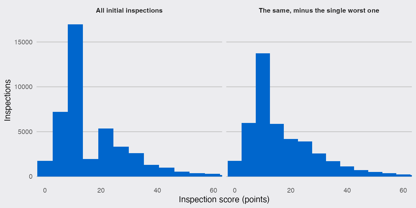
With all 43,278 inspections the bins are 5.41 points wide and one edge happens to land at 13.53, so the left panel shows a tall bar, a hole and a second hump, which reads like two kinds of restaurant. Remove one inspection and the maximum drops to 145, the bins become 5 points wide with an edge at 12.5, and the hole is gone: a smooth right-skewed hump that suggests nothing at all. Base R’s hist() is coarser still. Sturges’ rule gives bins 10 points wide, the (10, 20] bar holds 15,547 inspections against 14,124 in [0, 10], and the wall sits in the middle of a bar.
How do I choose the bin width for a histogram in R?
For integer data such as scores, ages or counts, give every value its own bar with geom_histogram(binwidth = 1) (or geom_bar(), which counts each distinct value). In ggplot2 4.0.3 a binwidth of 1 with no other arguments puts the edges at the half points, so each bar is centred on one integer and no value sits on an edge. The default bins = 30 spreads 30 equal bins between the minimum and the maximum, which is why a single extreme value can move every bar. For continuous data there is no single right width, so try a few and believe a feature only when it survives all of them.
ggplot(scores, aes(score, y = after_stat(density))) +   # binwidth 1: density = share
  geom_histogram(binwidth = 1, fill = dsp_colors[1]) +
  geom_vline(data = tibble(type = c("Initial inspection", "Re-inspection", "Re-inspection"),
                           cutoff = c(13.5, 13.5, 27.5)),
             aes(xintercept = cutoff), linetype = "dashed", color = "grey35") +
  geom_text(data = tibble(type  = rep(c("Initial inspection", "Re-inspection"), c(2, 3)),
                          score = c(6.5, 30, 6.5, 20.5, 34),
                          label = c("A", "no grade yet", "A", "B", "C")),
            aes(score, y = 0.155, label = label), inherit.aes = FALSE,
            fontface = "bold", color = "grey35") +
  facet_wrap(~ type, ncol = 1) +
  scale_y_continuous(labels = scales::label_percent()) +
  coord_cartesian(xlim = c(0, 45)) +
  labs(x = "Inspection score (points)", y = "Share of inspections") +
  dsp_theme
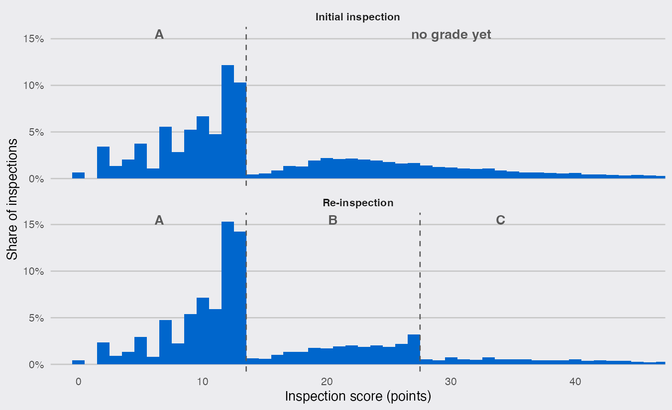
On initial inspections 12.2% scored 12 and 10.3% scored 13, so 23% landed on the last two scores that still earn an A, while 14, 15 and 16 together account for 1.8%. Put another way, 38% of the A grades handed out at an initial inspection went to a restaurant one or two points away from not getting one. The pile-up exists on inspection day: 97% of the 12s and 13s received their A the same day, so later hearings (the file’s scores are updated after adjudication) did not create it.
A score of 14 is not awkward to reach. Inspections with a single violation show what one violation is worth: 99.7% of them score between 2 and 10 points, with 5 (24%), 7 (11%) and 10 (10%) all common, so two violations can make 14 as 7 + 7, 10 + 4 or 9 + 5. Among the 12,947 initial inspections with exactly two violations, 34% scored 12 or 13 and 0.3% scored 14.
The wall appears only where a letter changes
Re-inspections carry a second cutoff that initial inspections do not: at a re-inspection, 28 points turns a B into a C, while at an initial inspection neither score decides a letter (anything above 13 means no grade yet and a re-inspection later). A re-inspection was 6.0 times as likely to score 27 as 28; an initial inspection was 1.2 times as likely, which is just the slope of the tail. At 13 against 14, which decides an A in both cases, the ratios are 23 on initial inspections and 22 on re-inspections. The scores bunch below a cutoff exactly where a letter depends on it, and nowhere else.
The file cannot say how an inspection ends up on the A side of the line. Most violations can be scored at several condition levels a point apart, and the inspector picks the level, so a point or two at the margin is within ordinary judgement and small nudges are enough to produce this shape. What the file does say is that the letter in the window is less precise than it looks: an A at 13 points and no A at 14 are one point apart, and far more restaurants sit on the A side of that point than the rest of the curve predicts. The histogram that shows it is the one with a bar for every score, not the default.


