
R 4.0.0 stopped turning strings into factors when you read a CSV, and I assumed that had quietly retired the oldest trap in R: calling as.numeric() on a factor and getting nonsense back. It has not retired. It moved. The import path is clean now, so the factors that reach your arithmetic arrive from somewhere else, and because the failure is silent I wanted to see what it actually costs on real data.
How do I convert a factor to a number in R?
Use as.numeric(as.character(f)), or the faster as.numeric(levels(f))[f] that ?factor recommends. Do not use as.numeric(f) on its own: on a factor that returns the internal level codes (1, 2, 3, …), not the values you can see, and it never warns you.
f <- factor(c("10", "2", "2", "33", "10"))

as.numeric(f)                    # 1 2 2 3 1  <- level codes, not values
## [1] 1 2 2 3 1
as.numeric(as.character(f))      # 10 2 2 33 10
## [1] 10  2  2 33 10
as.numeric(levels(f))[f]         # 10 2 2 33 10, and faster on long vectors
## [1] 10  2  2 33 10
That block runs on its own in base R, no packages needed. I checked it on R 4.6.1.
Why as.numeric() on a factor returns 1, 2, 3
A factor stores small integers plus a lookup table of labels, and as.numeric() hands you the integers. The codes follow the sorted order of the labels, and labels are text, so the sort is alphabetical rather than numeric. That is why "10" above becomes 1 and "2" becomes 2: the conversion is not even off by a constant, it reorders the values.
levels(f)          # "10" "2"  "33"  <- sorted as text
## [1] "10" "2"  "33"
as.integer(f)      # the stored codes
## [1] 1 2 2 3 1
Where factors still come from in R 4.x
Since R 4.0.0 (April 2020) read.csv() and data.frame() leave character columns as character, so that source is gone. These four still hand you a factor, and the first one is the one I keep meeting:
class(as.data.frame(table(c(1, 1, 2)))$Var1)   # table() counts -> factor
## [1] "factor"
class(cut(c(1, 5, 9), breaks = c(0, 3, 6, 10)))# binning -> factor
## [1] "factor"
class(factor(c(2020, 2021)))                   # explicit, often for plotting
## [1] "factor"
The fourth is .rds and .RData files saved before 2020, which still contain factors made under the old default. Survey imports are worth watching too: haven::as_factor() turns labelled SPSS and Stata columns into factors on purpose.
A wrong answer that looks like a right one
table() is the trap I care about, because counting something and then doing arithmetic on the counted values is an ordinary thing to want. I took every earthquake of magnitude 1.0 and above recorded in California in the first half of 2025, from the keyless USGS FDSN event API, and tabulated the magnitudes.
library(readr)
library(dplyr)

url <- paste0("https://earthquake.usgs.gov/fdsnws/event/1/query?format=csv",
              "&starttime=2025-01-01&endtime=2025-07-01",
              "&minlatitude=32.5&maxlatitude=42",
              "&minlongitude=-124.5&maxlongitude=-114",
              "&minmagnitude=1")
quakes <- read_csv(url, show_col_types = FALSE)

counts <- as.data.frame(table(round(quakes$mag, 1)))
names(counts) <- c("magnitude", "quakes")

head(counts, 3)
##   magnitude quakes
## 1         1   1160
## 2       1.1   2196
## 3       1.2   1158
class(counts$magnitude)
## [1] "factor"
trap    <- as.numeric(counts$magnitude)
correct <- as.numeric(as.character(counts$magnitude))

weighted.mean(trap,    counts$quakes)   # the trap
## [1] 5.713193
weighted.mean(correct, counts$quakes)   # the answer
## [1] 1.471427
mean(quakes$mag)                        # ground truth, straight from the raw data
## [1] 1.472809
Across 11,112 earthquakes the average magnitude is 1.47. The factor version says 5.71, and that is what makes it dangerous: 5.71 is a perfectly believable earthquake magnitude. Nothing about it says "this is a row number". The corrected version returns 1.47, matching the raw mean to within the width of one bin.
The same thing happens to a plot, and there it is even harder to catch, because the shape of the curve survives the mistake.
library(tidyr)
library(ggplot2)

dsp_colors <- c("#0066CC", "#E8862D", "#159A6C", "#7D5BD6",
                "#D64580", "#2AA9B8", "#C9A227")
dsp_theme <- theme_minimal(base_size = 13) +
  theme(plot.background    = element_rect(fill = "#ECECEF", color = NA),
        panel.background   = element_rect(fill = "#ECECEF", color = NA),
        panel.grid.minor   = element_blank(),
        panel.grid.major.x = element_blank(),
        panel.grid.major.y = element_line(color = "grey78"),
        axis.ticks         = element_blank(),
        plot.title         = element_text(face = "bold"),
        strip.text         = element_text(face = "bold"))

counts |>
  mutate(`as.numeric(magnitude): the level code` = trap,
         `as.numeric(as.character(magnitude)): the magnitude` = correct) |>
  pivot_longer(contains("as.numeric"), names_to = "conversion", values_to = "x") |>
  mutate(conversion = factor(conversion, levels = c(
    "as.numeric(magnitude): the level code",
    "as.numeric(as.character(magnitude)): the magnitude"))) |>
  ggplot(aes(x, quakes, color = conversion)) +
  geom_line(linewidth = 0.7) +
  geom_point(size = 1.4) +
  scale_y_log10() +
  scale_color_manual(values = dsp_colors[c(2, 1)]) +
  facet_wrap(~conversion, scales = "free_x") +
  labs(x = NULL, y = "earthquakes (log scale)",
       title = "Same counts, two different x axes") +
  dsp_theme +
  theme(legend.position = "none")
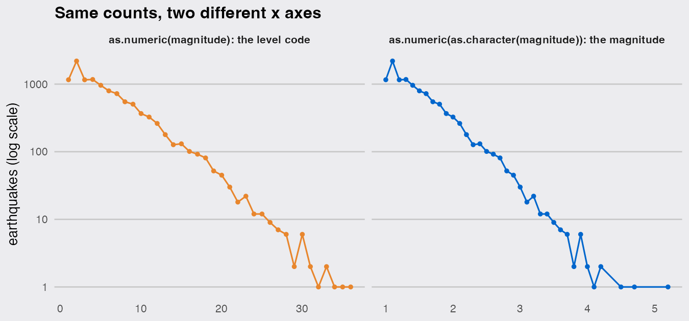
Both panels are the same 36 numbers. The left one is a plot you could publish without anyone blinking, and its x axis runs to 36 on a scale that stops at magnitude 5.2.
Rescaling the codes does not rescue it either. If you assume the codes are 0.1 apart and map code 1 back to magnitude 1, you get the right answer until the first magnitude that no earthquake reached: 7 bins in this window are empty, so 3 of the 36 rows land on the wrong magnitude, the worst of them off by 0.7 of a magnitude unit. table() only creates levels for values it saw, so the codes count observed bins, not steps along the scale.
The bug that passes your tests
The reason this survives code review is that on a factor of small whole numbers the codes and the values are often identical, so as.numeric() looks correct right up until the data changes underneath it.
rating <- factor(c(1, 2, 3, 4, 5))
as.numeric(rating)                          # 1 2 3 4 5, correct by coincidence
## [1] 1 2 3 4 5
kept <- droplevels(rating[rating != 2])     # drop the 2s and re-level
as.numeric(kept)                            # 1 2 3 4
## [1] 1 2 3 4
as.numeric(as.character(kept))              # 1 3 4 5
## [1] 1 3 4 5
Plain subsetting keeps every level, so as.numeric() stays accidentally right; droplevels(), a fresh factor() call, or a re-run of table() renumbers what is left and every value shifts. A filter added months later is enough to turn a passing pipeline into a wrong one, with no error and no warning.
One last case worth knowing: if the labels are not clean numbers, as.character() gives you NAs, and readr::parse_number() (readr 2.2.0) is the forgiving version.
money <- factor(c("1,200", "980", "3,500"))
as.numeric(as.character(money))     # NA 980 NA, with a coercion warning
## [1]  NA 980  NA
parse_number(as.character(money))   # 1200 980 3500
## [1] 1200  980 3500
My rule after this: if a column arrived from table(), cut(), an explicit factor(), or a file saved before 2020, run is.factor() on it before doing any arithmetic. It is the one class in R where the wrong answer is a plausible number rather than an error.

