
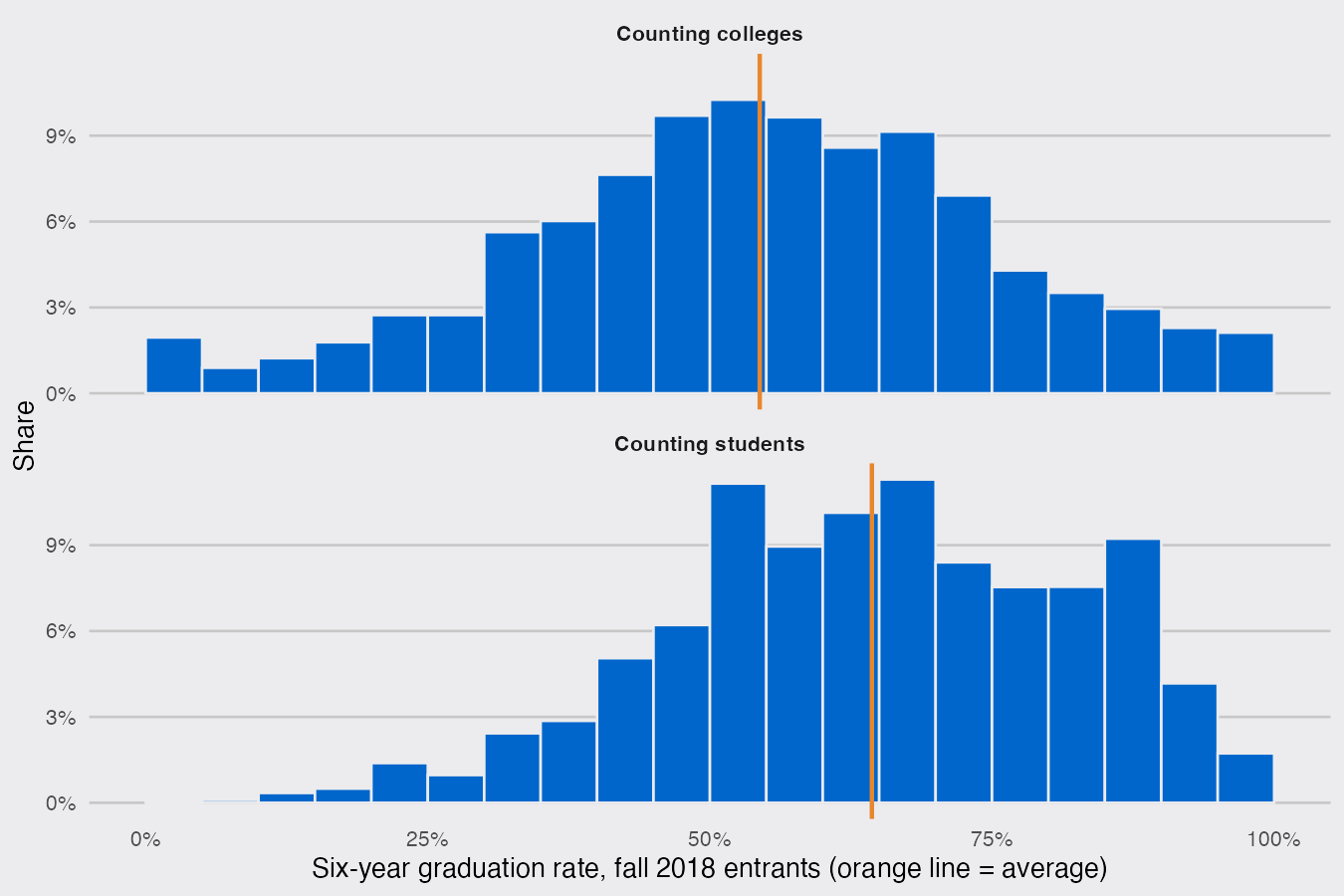
What share of students who start at a US four-year college finish a degree there? The Department of Education’s College Scorecard has a six-year graduation rate for every college, so the obvious move is mean() on that column. It returns 54.4%. Weighting each college by the number of students its rate describes returns 64.4%. Same column, 10 points apart, and both numbers are correct: the first describes the typical college, the second the typical student. I wanted to see where the gap comes from and what it does to comparisons between colleges. The short answer is that small colleges graduate fewer of their students, and that the gap between for-profit and public colleges nearly doubles once you count students instead of campuses.
Load the College Scorecard file
The June 2026 release has one row per institution and over 3,000 columns, so I read only the few I need. C150_4 is the share of first-time, full-time students who finished within six years (150% of the normal time) for the cohort that started in fall 2018, and D150_4 is the size of that cohort. I keep currently operating colleges that mainly award bachelor’s degrees (PREDDEG == 3). This runs with readr 2.2.0 and dplyr 1.2.1 on R 4.6.1:
library(tidyverse)

url <- "https://ed-public-download.scorecard.network/downloads/Most-Recent-Cohorts-Institution_06102026.zip"
zip <- tempfile(fileext = ".zip")
download.file(url, zip, mode = "wb", quiet = TRUE)

raw <- read_csv(unz(zip, "Most-Recent-Cohorts-Institution.csv"),
                col_select = c(INSTNM, CONTROL, PREDDEG, CURROPER, UGDS, C150_4, D150_4,
                               OMAWDP8_ALL, OMACHT8_FTFT, OMACHT8_PTFT,
                               OMACHT8_FTNFT, OMACHT8_PTNFT),
                na = c("", "NA", "NULL", "PrivacySuppressed"))  # replaces the default c("", "NA")

colleges <- raw |>
  filter(PREDDEG == 3, CURROPER == 1, !is.na(C150_4), D150_4 > 0) |>
  transmute(college    = INSTNM,
            control    = factor(CONTROL, 1:3, c("Public", "Private nonprofit", "For-profit")),
            grad_rate  = C150_4,
            cohort     = D150_4,
            undergrads = UGDS)
That leaves 1,794 colleges and the 1,613,174 students who started at them in 2018.
How do I average rates from groups of different sizes in R?
Weight each rate by the number of people it was computed on: weighted.mean(rate, n), which is the same number as pooling the counts, sum(rate * n) / sum(n). A plain mean(rate) gives every group one vote whatever its size. With three made-up colleges:
library(dplyr)

demo <- tibble(rate = c(0.40, 0.45, 0.85), n = c(50, 120, 9000))

demo |>
  summarise(per_college = mean(rate),
            per_student = weighted.mean(rate, n),
            pooled      = sum(rate * n) / sum(n))
## # A tibble: 1 × 3
##   per_college per_student pooled
##         <dbl>       <dbl>  <dbl>
## 1       0.567       0.842  0.842
Two traps while you are at it. In summarise(), a column created earlier is what later expressions see, so summarise(n = sum(n), wm = weighted.mean(rate, n)) stops with "’x’ and ‘w’ must have the same length": put the total last. And na.rm = TRUE drops missing rates but not missing weights, so a single NA weight makes the result NA.
Colleges versus students
On the real file, per college and per student, overall and by type of college:
colleges |>
  group_by(control) |>
  summarise(colleges    = n(),
            per_college = mean(grad_rate),
            per_student = weighted.mean(grad_rate, cohort),
            students    = sum(cohort))
## # A tibble: 3 × 5
##   control           colleges per_college per_student students
##   <fct>                <int>       <dbl>       <dbl>    <dbl>
## 1 Public                 568       0.530       0.635  1076739
## 2 Private nonprofit     1118       0.566       0.673   513890
## 3 For-profit             108       0.389       0.372    22545
39% of four-year colleges graduate fewer than half of their first-time students within six years, but those colleges took in only 20% of the students. The reason is size: graduation rates rise with the size of the entering class.
colleges |>
  mutate(size = cut(cohort, c(0, 100, 500, 2000, Inf), right = FALSE, dig.lab = 5)) |>
  group_by(size) |>
  summarise(colleges = n(), students = sum(cohort), grad_rate = mean(grad_rate)) |>
  mutate(share_colleges = colleges / sum(colleges),
         share_students = students / sum(students))
## # A tibble: 4 × 6
##   size       colleges students grad_rate share_colleges share_students
##   <fct>         <int>    <dbl>     <dbl>          <dbl>          <dbl>
## 1 [0,100)         346    10528     0.425          0.193        0.00653
## 2 [100,500)       664   191004     0.516          0.370        0.118
## 3 [500,2000)      562   556380     0.602          0.313        0.345
## 4 [2000,Inf)      222   855262     0.666          0.124        0.530
19% of these colleges started fewer than 100 first-time students in 2018 and graduate 43% of them on average, but together they hold 0.7% of the students. The 222 colleges that started 2,000 or more hold 53% of the students and graduate 67%. In mean() the long tail of small colleges outvotes the large ones, so the per-college figure lands closer to the small colleges’ rate.
The weighting moves public colleges from 53% to 64% and private nonprofits from 57% to 67%, but for-profits barely move (39% to 37%), because their large colleges do no better than their small ones. So the for-profit gap behind public colleges is 14 points per college and 26 points per student.
outcomes <- raw |>
  filter(PREDDEG == 3, CURROPER == 1, !is.na(OMAWDP8_ALL)) |>
  mutate(control  = factor(CONTROL, 1:3, c("Public", "Private nonprofit", "For-profit")),
         entrants = OMACHT8_FTFT + OMACHT8_PTFT + OMACHT8_FTNFT + OMACHT8_PTNFT) |>
  group_by(control) |>
  summarise(per_college = mean(OMAWDP8_ALL),
            per_student = weighted.mean(OMAWDP8_ALL, entrants))
oc <- \(who, col) outcomes[[col]][outcomes$control == who]
Six-year rates only follow first-time, full-time students, a small group at the large online for-profits. The Scorecard’s outcome measures follow everyone who started in 2016-17, part-time and transfer students included, for eight years. Counted that way, for-profits fall from 45% per college to 34% per student, and their gap behind public colleges widens from 13 to 29 points.
The weight aesthetic does the same thing for a histogram: aes(weight = cohort) makes each bar count students instead of colleges. You can copy the gray theme below for your own plots.
dsp_colors <- c("#0066CC", "#E8862D", "#159A6C", "#7D5BD6",
                "#D64580", "#2AA9B8", "#C9A227")
dsp_theme <- theme_minimal(base_size = 13) +
  theme(plot.background    = element_rect(fill = "#ECECEF", color = NA),
        panel.background   = element_rect(fill = "#ECECEF", color = NA),
        panel.grid.minor   = element_blank(),
        panel.grid.major.x = element_blank(),
        panel.grid.major.y = element_line(color = "grey78"),
        axis.ticks         = element_blank(),
        plot.title         = element_text(face = "bold"),
        strip.text         = element_text(face = "bold"))

views <- bind_rows(
  mutate(colleges, view = "Counting colleges", w = 1),
  mutate(colleges, view = "Counting students", w = cohort))

averages <- views |>
  group_by(view) |>
  summarise(avg = weighted.mean(grad_rate, w))

ggplot(views, aes(grad_rate, weight = w)) +
  geom_histogram(aes(y = after_stat(density * width)),   # share within each panel
                 binwidth = 0.05, boundary = 0, fill = dsp_colors[1], color = "#ECECEF") +
  geom_vline(data = averages, aes(xintercept = avg), color = dsp_colors[2], linewidth = 1) +
  facet_wrap(~ view, ncol = 1) +
  scale_x_continuous(labels = scales::percent) +
  scale_y_continuous(labels = scales::percent) +
  labs(x = "Six-year graduation rate, fall 2018 entrants (orange line = average)",
       y = "Share") +
  dsp_theme
Weight by the rate’s own denominator
The weight has to be the number of people the rate was computed on. Enrollment (UGDS) is the size column most people would reach for, and it gives 61.9% instead of 64.4%, because some very large colleges have tiny first-time, full-time cohorts. Arizona State University’s online campus has 53,782 undergraduates, a 2018 first-time, full-time cohort of 1 and a graduation rate of 0%; weighted by enrollment, that one student counts as 53,782 people who did not graduate. Capella University, 18,364 undergraduates and a cohort of 15, does the same to the for-profit figure, which drops to 32%. A quick check that the weight is right: weighted.mean(rate, n) should equal sum(rate * n) / sum(n) and describe a group of people you can name, here the 1,613,174 students who started in 2018.
Which number to report depends on the question. Describing or ranking colleges, average the colleges. Telling a student their odds, or describing what four-year colleges do for the people who enroll, pool the students: 64% of them graduate within six years, not 54%.

