
People often describe a region as "overdue" for a big earthquake, as if every quiet year added to a debt. I wondered whether the record backs that up, so I took all 1,620 magnitude 7+ earthquakes in the U.S. Geological Survey’s ComCat catalog since 1900 and checked whether the chance of the next one rises the longer a region has been quiet. It doesn’t. In the 33 regions with enough quakes to test, a region that had gone twice its usual gap without one had a 33% chance of a magnitude 7+ within the next half-gap. A region that had just had one: 43%. Pure chance with no memory predicts 39%, and a region running like even a loose clock would be at 77%.
How do I test whether an event is overdue in R?
Estimate a conditional probability: of all the waits that reached a given length, what share ended soon after? If an event really comes due, that share climbs with the time already waited. If it has no memory, the share stays flat. This block runs on its own as of R 4.6 and readr 2.2. USGS needs no key, and the file is under 300 KB.
library(tidyverse)

url <- paste0("https://earthquake.usgs.gov/fdsnws/event/1/query?format=csv",
              "&starttime=1900-01-01&endtime=2026-11-01",
              "&minmagnitude=7&eventtype=earthquake&orderby=time-asc")
quakes <- read_csv(url, show_col_types = FALSE)

# Of the waits that reached `quiet`, what share ended within `window`?
chance_next <- function(waits, quiet, window) {
  map(quiet, \(q) {
    reached <- waits[waits >= q]
    tibble(quiet = q, at_risk = length(reached), chance = mean(reached < q + window))
  }) |>
    list_rbind()
}

waits <- as.numeric(diff(quakes$time), units = "days")
chance_next(waits, quiet = c(0, 7, 14, 30, 60, 90), window = 14)
## # A tibble: 6 × 3
##   quiet at_risk chance
##   <dbl>   <int>  <dbl>
## 1     0    1619  0.428
## 2     7    1214  0.408
## 3    14     926  0.387
## 4    30     532  0.340
## 5    60     216  0.361
## 6    90      89  0.281
Worldwide, a magnitude 7+ comes about 12.8 times a year, 28.6 days apart on average. With no memory, the chance of another within 14 days is 38.7% however long the wait so far (1 - exp(-14 / mean(waits))). The catalog gives 42.8% right after a quake and 28.1% after 90 quiet days, though only 89 gaps got that far. Waiting longer did not raise it.
Why a flat global line proves nothing
That looks decisive and it isn’t. Merge many independent clocks onto one timeline and the combined gaps look random even when each clock is regular, so a global test comes out flat whatever single regions do (this is the Palm-Khintchine theorem). The test has to run inside regions, and it needs a check that it could detect a clock at all.
So I split the world into 20-degree boxes, keep the 33 with at least 10 gaps, and express each gap as a multiple of its own box’s average (the median box goes 4 years between quakes). For comparison I simulate a loose clock in each box, with the same average gap and a coefficient of variation of 0.5, the provisional generic value from a USGS recurrence study of 37 earthquake series. That study used a Brownian passage time distribution; I use a gamma, which has the same mean and spread and takes less code.
regional <- quakes |>
  mutate(region = paste(floor(latitude / 20), floor(longitude / 20))) |>
  mutate(gap = as.numeric(time - lag(time), units = "days"), .by = region) |>
  filter(!is.na(gap)) |>
  mutate(n_gaps = n(), mean_gap = mean(gap), x = gap / mean_gap, .by = region) |>
  filter(n_gaps >= 10)
span <- as.numeric(diff(range(quakes$time)), units = "days")

# One box: `clocks` independent gamma clocks, merged, each with a random start
clock_times <- function(mean_gap, clocks = 1, cv = 0.5) {
  shape <- 1 / cv^2
  gap <- mean_gap * clocks
  map(seq_len(clocks), \(i) {
    cumsum(rgamma(ceiling(span / gap) + 5, shape, shape / gap)) - runif(1, 0, gap)
  }) |>
    unlist() |>
    keep(\(t) t >= 0 & t <= span) |>
    sort()
}

simulate_clocks <- function(clocks = 1, reps = 200) {
  boxes <- distinct(regional, region, mean_gap)
  map(seq_len(reps), \(r) {
    mutate(boxes, rep = r, t = map(mean_gap, \(m) clock_times(m, clocks)))
  }) |>
    list_rbind() |>
    unnest(t)
}

per_region <- function(sim) {
  sim |>
    mutate(gap = t - lag(t), .by = c(rep, region)) |>
    filter(!is.na(gap)) |>
    mutate(x = gap / mean(gap), .by = c(rep, region))
}

set.seed(2026)
sim <- simulate_clocks()
clock_region <- per_region(sim)
clock_global <- sim |>
  arrange(rep, t) |>
  mutate(gap = t - lag(t), .by = rep) |>
  filter(!is.na(gap)) |>
  mutate(x = gap / mean(gap), .by = rep)
grid <- seq(0, 3, 0.25)
global_x <- waits / mean(waits)

# 95% band for the catalog: resample whole regions (or single gaps, globally)
band <- function(groups, B = 1000) {
  map(seq_len(B), \(i) {
    chance_next(unlist(sample(groups, replace = TRUE), use.names = FALSE), grid, 0.5)
  }) |>
    list_rbind() |>
    summarise(lo = quantile(chance, 0.025, na.rm = TRUE),
              hi = quantile(chance, 0.975, na.rm = TRUE), .by = quiet)
}

set.seed(2026)
curves <- bind_rows(
  chance_next(global_x, grid, 0.5) |> left_join(band(as.list(global_x)), by = "quiet") |>
    mutate(source = "catalog", view = "One global timeline"),
  chance_next(regional$x, grid, 0.5) |> left_join(band(split(regional$x, regional$region)), by = "quiet") |>
    mutate(source = "catalog", view = "Region by region"),
  chance_next(clock_global$x, grid, 0.5) |> mutate(source = "clock", view = "One global timeline"),
  chance_next(clock_region$x, grid, 0.5) |> mutate(source = "clock", view = "Region by region")
)
dsp_colors <- c("#0066CC", "#E8862D", "#159A6C", "#7D5BD6",
                "#D64580", "#2AA9B8", "#C9A227")
dsp_theme <- theme_minimal(base_size = 13) +
  theme(plot.background    = element_rect(fill = "#ECECEF", color = NA),
        panel.background   = element_rect(fill = "#ECECEF", color = NA),
        panel.grid.minor   = element_blank(),
        panel.grid.major.x = element_blank(),
        panel.grid.major.y = element_line(color = "grey78"),
        axis.ticks         = element_blank(),
        plot.title         = element_text(face = "bold"),
        strip.text         = element_text(face = "bold"))

labels <- tribble(
  ~view,                 ~quiet, ~chance, ~source,   ~label,
  "One global timeline", 2.20,   0.55,    "clock",   "if regions ran like clocks",
  "One global timeline", 1.10,   0.22,    "catalog", "USGS catalog",
  "Region by region",    1.95,   0.90,    "clock",   "if regions ran like clocks",
  "Region by region",    1.50,   0.20,    "catalog", "USGS catalog"
)
no_memory_label <- tibble(view = "One global timeline", quiet = 0.85, chance = 0.62,
                          label = "dashed line: no memory")

ggplot(curves, aes(quiet, chance, color = source, fill = source)) +
  geom_hline(yintercept = 1 - exp(-0.5), linetype = "dashed", color = "grey40") +
  geom_ribbon(aes(ymin = lo, ymax = hi), alpha = 0.2, color = NA) +
  geom_line(linewidth = 1) +
  geom_text(data = labels, aes(label = label), size = 3.8, fontface = "bold") +
  geom_text(data = no_memory_label, aes(quiet, chance, label = label), inherit.aes = FALSE,
            size = 3.4, color = "grey30") +
  facet_wrap(~view) +
  scale_color_manual(values = c(catalog = dsp_colors[1], clock = dsp_colors[2])) +
  scale_fill_manual(values = c(catalog = dsp_colors[1], clock = dsp_colors[2])) +
  scale_y_continuous(labels = scales::percent, limits = c(0, 1)) +
  labs(title = "A clock only shows up when you look region by region",
       x = "Time already quiet, as a multiple of the usual gap",
       y = "Chance of a magnitude 7+\nin the next half-gap") +
  dsp_theme +
  theme(legend.position = "none", panel.spacing = unit(1.5, "lines"))
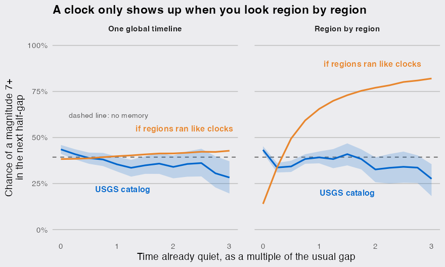
On one timeline the two cannot be told apart: up to twice the usual gap the simulated clocks stay between 38% and 41%, and the catalog between 34% and 44%. Region by region they split. The clocks climb from 14% right after a quake to 77% at twice the usual gap. The catalog does the opposite: it starts at its highest, 43%, as aftershocks and paired ruptures land soon after a quake, then settles between 33% and 41% and stays there.
How do I summarize waiting times with survreg()?
Fit survreg(Surv(x) ~ 1, dist = "weibull") and read the shape as 1 / fit$scale: above 1 the chance rises with time waited, below 1 it falls, and exactly 1 is no memory. survreg() ships with R in the survival package (3.8 here).
library(survival)

fit <- survreg(Surv(x) ~ 1, data = regional, dist = "weibull",
               cluster = region, robust = TRUE)
shape <- 1 / fit$scale
ci <- exp(-log(fit$scale) + c(-1.96, 1.96) * sqrt(vcov(fit)[2, 2]))
clock_shape <- 1 / survreg(Surv(x) ~ 1, data = clock_region, dist = "weibull")$scale

round(c(catalog = shape, lower = ci[1], upper = ci[2], clocks = clock_shape), 2)
## catalog   lower   upper  clocks
##    0.73    0.68    0.78    2.15
The catalog’s shape is 0.73, and the 95% interval, clustered on region, runs from 0.68 to 0.78. The clocks come out at 2.15.
What this does not rule out
Aftershocks pull the early chance up, so they could be hiding a rising line. Keeping only gaps longer than a year, the catalog stays flat at 52% at half a gap and 54% at twice, while the clocks under the same filter climb from 56% to 81%. The answer also held with 5, 10 and 30-degree boxes and when starting from 1950 or 1973, since early magnitudes are rougher: Weibull shapes ran from 0.63 to 0.74.
The limit is the box. A 20-degree box is about 2,200 km tall and holds many fault segments, and merging happens inside it too: with 4 independent clocks per box (simulate_clocks(clocks = 4)) the line would still reach 54% at twice the usual gap, but with 12 it reaches only 44%, close to the no-memory line, and a box that size can hold more rupture segments than that. So this rules out region-wide clocks, not a single fault segment that ruptures every few centuries, which a 127-year catalog could not see repeat anyway.
It also does not make a quiet region safe. The flat line sits well above zero: in the median box, roughly a one-in-three chance of a magnitude 7+ every two years. What the record supports is narrower: the chance peaks just after a quake, and after that the calendar tells you nothing.
