
I pulled a month of hourly temperatures from a weather API, grouped them by day with as.Date(), and got a daily maximum for Phoenix that was 5.1 degrees Celsius hotter than the day had actually been. Nothing errored, nothing warned, and the number looked entirely plausible for July in Arizona.
The reason is a default I had never read: a calendar date is not a property of an instant, it depends on the time zone you ask in, and as.Date() always asks in UTC.
Why does as.Date() give the wrong day in R?
Because as.Date() on a POSIXct converts the instant to UTC before it drops the clock time, whatever time zone the object itself carries. The method signature is as.Date(x, tz = "UTC", ...), so the day boundary is UTC midnight unless you say otherwise.
library(lubridate)

x <- as.POSIXct("2026-01-01 20:00:00", tz = "America/Chicago")

format(x, "%Y-%m-%d %H:%M %Z")  # the instant, on a Chicago wall clock
## [1] "2026-01-01 20:00 CST"
as.Date(x)                # base R: converted to UTC first
## [1] "2026-01-02"
as.Date(x, tz = "America/Chicago")
## [1] "2026-01-01"
as_date(x)                # lubridate: uses the object's own zone
## [1] "2026-01-01"
Eight in the evening in Chicago is already the next day in UTC, so as.Date() returns 2 January for a timestamp whose printed representation says 1 January. Worth noting for anyone who mixes the two: on the same object, base R’s as.Date() and lubridate’s as_date() return different dates, and both are behaving as documented (R 4.6.1, lubridate 1.9.5).
Getting the calendar date you actually meant
Pass tz explicitly, and pass the zone the data is about, not the zone your laptop happens to be in.
as.Date(x, tz = "America/Chicago")              # base R
## [1] "2026-01-01"
as_date(with_tz(x, "America/Chicago"))          # lubridate
## [1] "2026-01-01"
floor_date(with_tz(x, "America/Chicago"), "day")  # keeps it a POSIXct
## [1] "2026-01-01 CST"
with_tz() changes the zone the instant is displayed in without moving the instant, which is why it composes safely with anything downstream. Use floor_date() when you want to keep sub-day resolution available, for example to group by hour later in the same pipeline.
Do not reach for the arithmetic shortcut instead. Subtracting the offset by hand, x - hours(6), is right for this January timestamp and wrong for the same script in July: Chicago is six hours behind UTC in winter and five in summer, so a hardcoded offset silently mislabels half the year. Name the zone and let the time zone database do the arithmetic, OlsonNames() lists the names R accepts.
What it costs on real data
Here is the case that caught me. Open-Meteo’s historical weather API is keyless and returns hourly values in UTC by default, so the timestamps arrive correct and the tempting next step is as.Date().
library(tidyverse)
library(jsonlite)

url <- paste0("https://archive-api.open-meteo.com/v1/archive?latitude=33.4484&longitude=-112.0740",
              "&start_date=2026-06-30&end_date=2026-08-01&hourly=temperature_2m&timezone=GMT")
j <- fromJSON(url)

phx <- tibble(time_utc = ymd_hm(j$hourly$time, tz = "UTC"),
              temp_c   = j$hourly$temperature_2m) |>
  mutate(utc_day   = as.Date(time_utc),
         local_day = as.Date(time_utc, tz = "America/Phoenix"))

mean(phx$utc_day != phx$local_day)
## [1] 0.2916667
Phoenix sits at UTC-7 all year, since Arizona does not observe daylight saving time, so 29.2% of the hourly readings, seven hours out of every twenty-four, are filed under a different calendar date by the two columns. A UTC day in Phoenix runs from 17:00 one afternoon to 17:00 the next.
daily <- phx |>
  pivot_longer(c(utc_day, local_day), names_to = "grouping", values_to = "day") |>
  mutate(grouping = str_remove(grouping, "_day")) |>
  group_by(grouping, day) |>
  summarise(tmax = max(temp_c), hours = n(), .groups = "drop") |>
  filter(hours == 24, between(day, as.Date("2026-07-01"), as.Date("2026-07-31"))) |>
  select(-hours) |>
  pivot_wider(names_from = grouping, values_from = tmax) |>
  mutate(gap = utc - local)

daily |> filter(gap != 0) |> arrange(desc(abs(gap)))
## # A tibble: 16 × 4
##    day        local   utc    gap
##    <date>     <dbl> <dbl>  <dbl>
##  1 2026-07-16  36.3  41.4  5.1
##  2 2026-07-28  40.3  43.1  2.80
##  3 2026-07-17  32.1  34.4  2.30
##  4 2026-07-04  38.5  40.6  2.10
##  5 2026-07-21  38.2  40    1.80
##  6 2026-07-18  33.8  32.1 -1.70
##  7 2026-07-19  37.8  36.7 -1.10
##  8 2026-07-15  41.4  40.4 -1
##  9 2026-07-11  41.8  42.7  0.900
## 10 2026-07-13  40.7  41.3  0.600
## 11 2026-07-10  43.2  43.7  0.5
## 12 2026-07-12  41.3  41.8  0.5
## 13 2026-07-25  45.3  45.8  0.5
## 14 2026-07-29  42.5  42.2 -0.300
## 15 2026-07-01  37.4  37.6  0.200
## 16 2026-07-14  40.4  40.2 -0.200
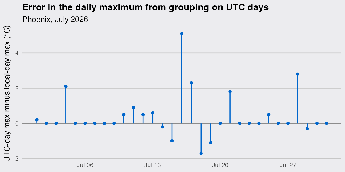
16 of the 31 daily maxima change, the largest by 5.1 degrees on 16 July. Counting days at or above 43 degrees Celsius, the UTC grouping gives 12 and the honest one gives 11. Neither version is flagged as suspect anywhere in the pipeline.
The mechanism is easiest to see on the worst day. The maximum that as.Date() attributes to 16 July was measured at 18:00 on 15 July, an hour after the UTC day rolled over.
dsp_colors <- c("#0066CC", "#E8862D", "#159A6C", "#7D5BD6",
                "#D64580", "#2AA9B8", "#C9A227")
dsp_theme <- theme_minimal(base_size = 13) +
  theme(plot.background    = element_rect(fill = "#ECECEF", color = NA),
        panel.background   = element_rect(fill = "#ECECEF", color = NA),
        panel.grid.minor   = element_blank(),
        panel.grid.major.x = element_blank(),
        panel.grid.major.y = element_line(color = "grey78"),
        axis.ticks         = element_blank(),
        plot.title         = element_text(face = "bold"),
        strip.text         = element_text(face = "bold"))

phx_local <- function(s) as.POSIXct(s, tz = "America/Phoenix")

win <- phx |>
  filter(between(time_utc, phx_local("2026-07-15 00:00"), phx_local("2026-07-17 23:00"))) |>
  mutate(local_time = with_tz(time_utc, "America/Phoenix"))

peaks <- bind_rows(
  win |> filter(utc_day   == as.Date("2026-07-16")) |> slice_max(temp_c, n = 1) |> mutate(lab = "max of the UTC day"),
  win |> filter(local_day == as.Date("2026-07-16")) |> slice_max(temp_c, n = 1) |> mutate(lab = "max of the Phoenix day"))

ggplot(win, aes(local_time, temp_c)) +
  annotate("rect", xmin = phx_local("2026-07-15 17:00"), xmax = phx_local("2026-07-16 17:00"),
           ymin = -Inf, ymax = Inf, fill = dsp_colors[2], alpha = .12) +
  geom_vline(xintercept = phx_local(c("2026-07-16 00:00", "2026-07-17 00:00")),
             color = "grey60", linewidth = .4) +
  geom_line(color = dsp_colors[1], linewidth = .7) +
  geom_point(data = peaks, aes(color = lab), size = 3) +
  scale_color_manual(values = c("max of the Phoenix day" = dsp_colors[3],
                                "max of the UTC day"     = dsp_colors[5]), name = NULL) +
  labs(title = "Two different maxima for 16 July in Phoenix",
       subtitle = "Shaded band: the UTC day. Grey lines: local midnight.",
       x = NULL, y = "Temperature (°C)") +
  dsp_theme + theme(legend.position = "top")
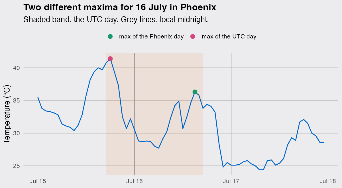
Across the month the error is not a rounding wobble, and it has a sign: on days when the previous evening was hotter than the afternoon that followed, the UTC grouping inherits the older, hotter reading.
ggplot(daily, aes(day, gap)) +
  geom_hline(yintercept = 0, color = "grey55") +
  geom_segment(aes(xend = day, yend = 0), color = dsp_colors[1], linewidth = .8) +
  geom_point(color = dsp_colors[1], size = 1.8) +
  labs(title = "Error in the daily maximum from grouping on UTC days",
       subtitle = "Phoenix, July 2026",
       x = NULL, y = "UTC-day max minus local-day max (°C)") +
  dsp_theme
The other half of the trap
The same question, which zone, decides what as.POSIXct() does with a string that has no offset. With no tz argument it uses the machine’s zone, so a script that parses "2026-07-01 20:00:00" produces a different instant, and sometimes a different date, on a colleague’s laptop than on yours.
tz_was <- Sys.getenv("TZ")

Sys.setenv(TZ = "America/Chicago")
as.Date(as.POSIXct("2026-07-01 20:00:00"))
## [1] "2026-07-02"
Sys.setenv(TZ = "Europe/Berlin")
as.Date(as.POSIXct("2026-07-01 20:00:00"))
## [1] "2026-07-01"
if (tz_was == "") Sys.unsetenv("TZ") else Sys.setenv(TZ = tz_was)
Two machines, one string, two dates, and no warning on either. This matters more than the date, because parsing a local wall clock as UTC misplaces the instant itself, and with_tz() will not repair it: it re-displays the same instant somewhere else. force_tz() is the repair, keeping the clock reading and changing only the label.
bad <- ymd_hms("2026-07-01 20:00:00")     # ymd_hms() defaults to UTC
with_tz(bad,  "America/Chicago")          # same instant, Chicago clock
## [1] "2026-07-01 15:00:00 CDT"
force_tz(bad, "America/Chicago")          # same clock, Chicago instant
## [1] "2026-07-01 20:00:00 CDT"
readr::read_csv() has the same default, so a column of naive local timestamps comes back labelled UTC without comment. The habit that closes all of this is the same one: name the time zone at the point where a string becomes a timestamp, and name it again at the point where a timestamp becomes a date.
