
I joined two country tables on their ISO code, which is meant to be the safe key, and got back more rows than I put in. That kind of surprise is at least loud. What stayed with me was the second version of the same mistake: the row count came back exactly right, nothing warned, and fifteen rows were quietly holding somebody else’s number.
Both come from one rule that I had never seen written down anywhere I was likely to read it. In R, a missing value is a join key. NA matches NA, so every row whose key is blank matches every other row whose key is blank. SQL does the opposite, since NULL = NULL is never true there, and I suspect that is where most people’s expectation comes from.
Below I take a real pair of tables, watch both failure modes happen, measure what they cost, and end with the guards that turn a join into something that fails loudly instead.
Two tables and an obvious key
I am using two indicators from Our World in Data: life expectancy at birth and median age. Both come down as plain CSV with no key or registration, and both are shaped the same way: one row per entity per year, with an entity name and a code.
library(readr)
library(dplyr)
library(ggplot2)

owid <- function(slug) {
  read_csv(paste0("https://ourworldindata.org/grapher/", slug,
                  ".csv?v=1&csvType=full&useColumnShortNames=true"),
           show_col_types = FALSE, progress = FALSE)
}

life <- owid("life-expectancy") |>
  rename(life_exp = life_expectancy_0) |>
  filter(year == 2023) |>
  select(entity, code, life_exp)

age <- owid("median-age") |>
  rename(median_age = median_age__sex_all__age_all__variant_estimates) |>
  filter(year == 2023, !is.na(median_age)) |>
  select(entity, code, median_age)

c(life = nrow(life), age = nrow(age))
## life  age
##  261  253
The code column is ISO 3166 alpha-3 for countries, plus a handful of OWID_ codes for things the standard does not cover. It is the column you are supposed to join on, precisely because country names are a mess across providers. Here is the part that matters:
life |> filter(is.na(code)) |> pull(entity) |> head(6)
## [1] "Americas"
## [2] "High-and-upper-middle-income countries"
## [3] "Land-locked Developing Countries (LLDC)"
## [4] "Latin America and the Caribbean"
## [5] "Least developed countries"
## [6] "Less developed regions"
c(blank_in_life = sum(is.na(life$code)), blank_in_age = sum(is.na(age$code)))
## blank_in_life  blank_in_age
##            15             5
Neither table is broken. Both simply carry aggregate rows next to the country rows, and an aggregate like "Least developed countries" has no ISO code to put in the column, so the field is empty. Almost every statistical source I have pulled does this somewhere: a total row, a regional subtotal, a category that predates the code list.
The join grows
say_warnings <- function(expr) {
  withCallingHandlers(expr, warning = function(w) {
    cat("Warning:", conditionMessage(w), "\n")
    invokeRestart("muffleWarning")
  })
}

joined <- say_warnings(
  left_join(life, age, by = "code", suffix = c("_life", "_age"))
)
## Warning: Detected an unexpected many-to-many relationship between `x` and `y`.
## ℹ Row 6 of `x` matches multiple rows in `y`.
## ℹ Row 122 of `y` matches multiple rows in `x`.
## ℹ If a many-to-many relationship is expected, set `relationship =
##   "many-to-many"` to silence this warning.
c(rows_in = nrow(life), rows_out = nrow(joined))
##  rows_in rows_out
##      261      321
A left join is supposed to return one row per row of life. It returned 321 from 261. Since dplyr 1.1.0 there is at least a warning, and it is a good one, but it arrives phrased as a relationship problem rather than as a missing-value problem, so it is easy to read it as "these two tables just overlap in a complicated way" and move on.
The extra rows are not complicated at all:
joined |>
  filter(is.na(code)) |>
  select(entity_life, entity_age, life_exp, median_age) |>
  head(5)
## # A tibble: 5 × 4
##   entity_life entity_age                                     life_exp median_age
##   <chr>       <chr>                                             <dbl>      <dbl>
## 1 Americas    Least developed countries                          77.3       19.2
## 2 Americas    Less developed regions                             77.3       28.4
## 3 Americas    Less developed regions, excluding China            77.3       25.6
## 4 Americas    Less developed regions, excluding least devel…     77.3       30.6
## 5 Americas    More developed regions                             77.3       41.6
15 blank-code rows on the left met 5 blank-code rows on the right and produced every combination, 75 rows in which the life expectancy of one aggregate sits beside the median age of a different one. "Americas" paired with "Least developed countries" is not a data quality issue in either source. It is a row that R invented during the join.
Why NA matches NA
The behavior is a documented default rather than an accident. Every dplyr join takes an na_matches argument, and it is set to "na":
x <- tibble(code = c("AFG", NA, NA), v = 1:3)
y <- tibble(code = c("AFG", NA),     w = c(10, 20))

left_join(x, y, by = "code")                        # default: na_matches = "na"
## # A tibble: 3 × 3
##   code      v     w
##   <chr> <int> <dbl>
## 1 AFG       1    10
## 2 <NA>      2    20
## 3 <NA>      3    20
left_join(x, y, by = "code", na_matches = "never")
## # A tibble: 3 × 3
##   code      v     w
##   <chr> <int> <dbl>
## 1 AFG       1    10
## 2 <NA>      2    NA
## 3 <NA>      3    NA
This is not a tidyverse quirk either. Base R agrees, and has its own spelling of the fix:
merge(x, y, by = "code", all.x = TRUE)
##   code v  w
## 1  AFG 1 10
## 2 <NA> 2 20
## 3 <NA> 3 20
merge(x, y, by = "code", all.x = TRUE, incomparables = NA)
##   code v  w
## 1  AFG 1 10
## 2 <NA> 2 NA
## 3 <NA> 3 NA
Which default is right depends on what the NA means to you. If it is a real category, "the unclassified group", then matching it to itself is sensible. If it means "we do not know what this is", then two unknowns are not evidence of a match, and R’s default is doing something you almost never want. In my experience with data pulled from public sources, blank keys are the second kind essentially every time.
The version that leaves no trace
The warning above only fires because both sides had several blank-code rows. Watch what happens when the lookup table has exactly one, which is what you get from any source carrying a single "World" or "Total" row.
lookup <- age |> filter(!is.na(code) | entity == "More developed regions")
sum(is.na(lookup$code))
## [1] 1
quiet <- say_warnings(
  left_join(life, lookup, by = "code", suffix = c("_life", "_age"))
)

c(rows_in = nrow(life), rows_out = nrow(quiet))
##  rows_in rows_out
##      261      261
No warning. No change in row count. The join is now many-to-one, which is exactly the relationship a left join is meant to have, so there is nothing for dplyr to object to. And yet:
quiet |>
  filter(is.na(code)) |>
  select(entity_life, entity_age, median_age) |>
  head(5)
## # A tibble: 5 × 3
##   entity_life                             entity_age             median_age
##   <chr>                                   <chr>                       <dbl>
## 1 Americas                                More developed regions       41.6
## 2 High-and-upper-middle-income countries  More developed regions       41.6
## 3 Land-locked Developing Countries (LLDC) More developed regions       41.6
## 4 Latin America and the Caribbean         More developed regions       41.6
## 5 Least developed countries               More developed regions       41.6
Every one of the 15 blank-code rows on the left has been handed a median age of 41.6 years, the value belonging to "More developed regions". "Least developed countries" now carries the median age of the developed world. Nothing in the object tells you this happened. The row count, which is the check most of us actually run, agrees with the input and always will.
Here is what those rows look like once they are in a plot, alongside the real matches:
dsp_colors <- c("#0066CC", "#E8862D", "#159A6C", "#7D5BD6",
                "#D64580", "#2AA9B8", "#C9A227")
dsp_theme <- theme_minimal(base_size = 13) +
  theme(plot.background    = element_rect(fill = "#ECECEF", color = NA),
        panel.background   = element_rect(fill = "#ECECEF", color = NA),
        panel.grid.minor   = element_blank(),
        panel.grid.major.x = element_blank(),
        panel.grid.major.y = element_line(color = "grey78"),
        axis.ticks         = element_blank(),
        plot.title         = element_text(face = "bold"),
        strip.text         = element_text(face = "bold"))

quiet |>
  filter(!is.na(median_age)) |>
  mutate(kind = if_else(is.na(code), "Given a value that is not theirs", "Real matches")) |>
  ggplot(aes(median_age, life_exp, color = kind)) +
  geom_point(size = 1.9, alpha = 0.85) +
  scale_color_manual(values = c("Real matches" = dsp_colors[1],
                                "Given a value that is not theirs" = dsp_colors[2])) +
  labs(title = "No warning, no extra rows, fifteen wrong values",
       subtitle = "One blank-code row in the lookup table is enough",
       x = "Median age (years)", y = "Life expectancy at birth (years)",
       color = NULL) +
  dsp_theme + theme(legend.position = "top")
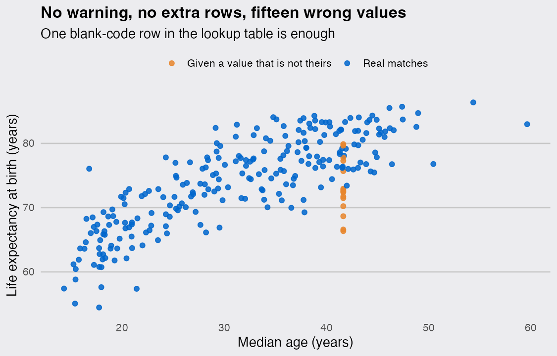
The wrong rows land in the middle of the cloud, at a median age that is perfectly plausible for a rich country. Without the color there is nothing to see. This is the case I now actively check for, because the loud version at least stops you.
What the extra rows cost
Back to the first join, the one that grew. If I go on to ask how life expectancy tracks median age across the world in 2023, the invented rows come along.
is_country <- function(code) !is.na(code) & (nchar(code) == 3 | code == "OWID_KOS")

as_returned <- joined |> filter(!is.na(median_age))
countries   <- as_returned |> filter(is_country(code))

fit_summary <- function(d, label) {
  m <- lm(life_exp ~ median_age, data = d)
  tibble(table = label,
         rows  = nrow(d),
         slope = round(coef(m)[["median_age"]], 3),
         r     = round(cor(d$life_exp, d$median_age), 3),
         r2    = round(summary(m)$r.squared, 3))
}

bind_rows(fit_summary(as_returned, "join as returned"),
          fit_summary(countries,   "countries only"))
## # A tibble: 2 × 5
##   table             rows slope     r    r2
##   <chr>            <int> <dbl> <dbl> <dbl>
## 1 join as returned   317 0.504 0.727 0.528
## 2 countries only     237 0.592 0.826 0.682
80 of the 317 rows I would have modeled, 25 percent of the sample, are aggregates or invented pairs. They pull the correlation from 0.826 down to 0.727 and flatten the slope from 0.592 to 0.504 years of life expectancy per year of median age. Nothing about those numbers looks wrong on its own. A correlation of 0.727 is the sort of figure you would write into a paragraph without a second thought.
as_returned |>
  mutate(kind = if_else(is.na(code), "Invented pairs (blank code)", "Real matches")) |>
  ggplot(aes(median_age, life_exp)) +
  geom_point(aes(color = kind), size = 1.9, alpha = 0.85) +
  geom_smooth(data = countries, method = "lm", formula = y ~ x, se = FALSE,
              color = dsp_colors[1], linewidth = 0.9) +
  geom_smooth(method = "lm", formula = y ~ x, se = FALSE,
              color = dsp_colors[2], linewidth = 0.9, linetype = "22") +
  scale_color_manual(values = c("Real matches" = dsp_colors[1],
                                "Invented pairs (blank code)" = dsp_colors[2])) +
  labs(title = "Seventy-five rows that match nothing real",
       subtitle = "Dashed line: the fit on the joined table exactly as it came back",
       x = "Median age (years)", y = "Life expectancy at birth (years)",
       color = NULL) +
  dsp_theme + theme(legend.position = "top")
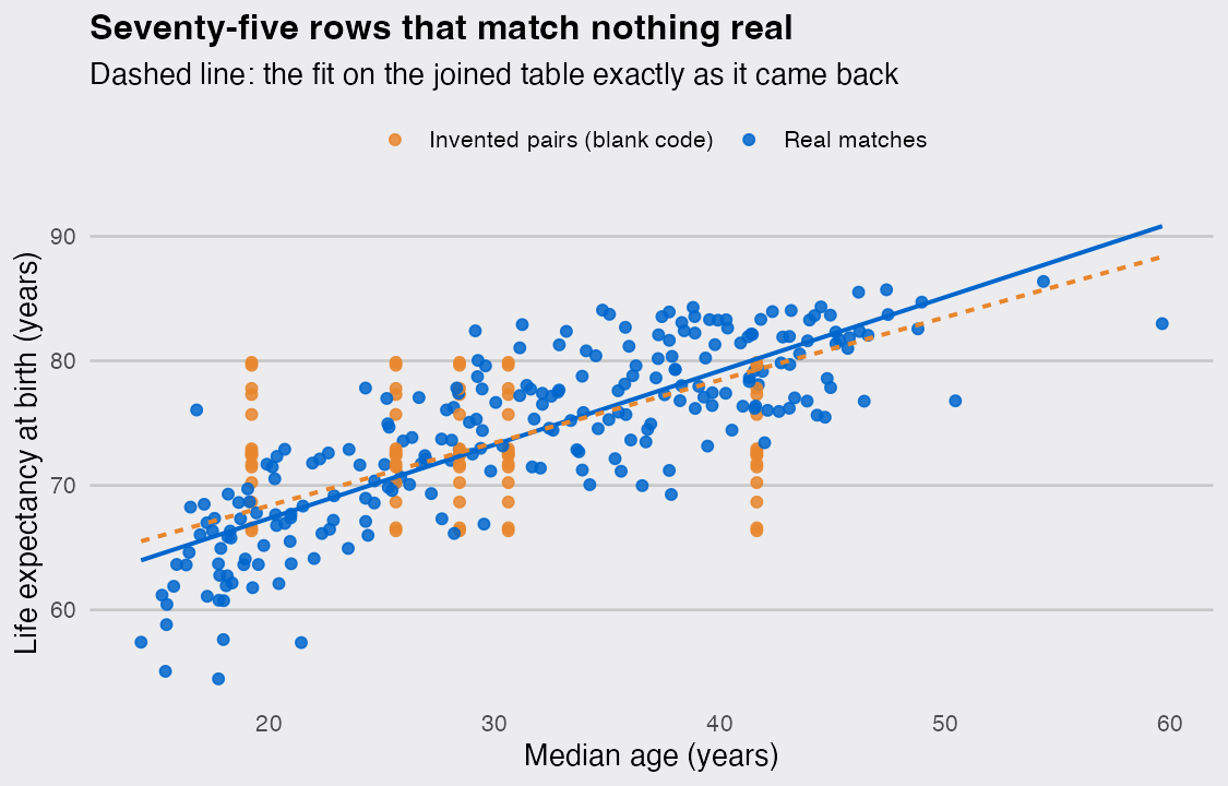
The orange points form vertical stripes, one per distinct blank-code value on the right-hand side, each stripe stacking every blank-code value from the left. That signature is worth memorizing. Whenever a scatter plot of joined data shows a few suspiciously straight vertical or horizontal lines of points, a key matched more rows than it should have.
Writing the join as a contract
The fix is not to remember any of this. It is to say out loud what the join is supposed to do, and let R refuse when it cannot. na_matches has been there all along, and dplyr 1.1.0 added the rest.
try_join <- function(expr) {
  out <- tryCatch(expr, error = function(e) conditionMessage(e))
  if (is.character(out)) cat("Error:", out, "\n") else cat("Returned", nrow(out), "rows\n")
}

# What I actually mean: each country on the left gets at most one match,
# blanks match nothing, and I want to hear about it if that is not true.
try_join(
  left_join(life, age, by = "code",
            na_matches   = "never",
            relationship = "many-to-one")
)
## Returned 261 rows
# The same join without the na_matches guard still cannot hold.
try_join(
  left_join(life, age, by = "code", relationship = "many-to-one")
)
## Error: Each row in `x` must match at most 1 row in `y`.
## ℹ Row 6 of `x` matches multiple rows in `y`.
Three arguments I now write by default:
na_matches = "never"makes blank keys match nothing, which is the SQL behavior and, I would argue, the useful one for keys pulled from files.relationship =states the cardinality you believe in ("one-to-one","many-to-one","one-to-many") and errors instead of silently multiplying rows. This is the argument that catches the quiet case above, because "many-to-one" is not violated by a bad NA match, but "one-to-one" is.unmatched = "error"turns unmatched keys into a failure rather than a column ofNA. In a left join it checksy, since rows ofxare kept by definition.
The last guard is not an argument at all. Before trusting a lookup table, look at what will not match:
unmatched <- anti_join(life, age, by = "code", na_matches = "never")
unmatched |> select(entity, code) |> print(n = Inf)
## # A tibble: 19 × 2
##    entity                                                      code
##    <chr>                                                       <chr>
##  1 Africa                                                      OWID_AFR
##  2 Americas                                                    <NA>
##  3 Asia                                                        OWID_ASI
##  4 Europe                                                      OWID_EUR
##  5 High-and-upper-middle-income countries                      <NA>
##  6 Land-locked Developing Countries (LLDC)                     <NA>
##  7 Latin America and the Caribbean                             <NA>
##  8 Least developed countries                                   <NA>
##  9 Less developed regions                                      <NA>
## 10 Less developed regions, excluding China                     <NA>
## 11 Less developed regions, excluding least developed countries <NA>
## 12 Low-and-Lower-middle-income countries                       <NA>
## 13 Low-and-middle-income countries                             <NA>
## 14 Middle-income countries                                     <NA>
## 15 More developed regions                                      <NA>
## 16 No income group available                                   <NA>
## 17 Northern America                                            <NA>
## 18 Oceania                                                     OWID_OCE
## 19 Small Island Developing States (SIDS)                       <NA>
That list is the join’s own account of itself, and it is the step I would keep if I had to drop the other three. Every row on it is an aggregate, which is the answer I want: the blanks that caused all the trouble, plus four continents that one file codes and the other does not carry. No actual country is being dropped, and that is a claim I can check rather than assume.
unmatched |> filter(is_country(code)) |> nrow()
## [1] 0
When that number is not zero, the useful question is never "how many rows did I lose" but "what do the lost rows have in common". Dropped rows are hardly ever a random sample. They are the small territories, the renamed states, the entities one provider counts and the other does not.
With the guards in place the analysis is the boring one I meant to run in the first place:
panel <- inner_join(
  life |> filter(is_country(code)),
  age  |> filter(is_country(code)),
  by = "code", na_matches = "never", relationship = "one-to-one",
  suffix = c("", "_age")
)

nrow(panel)
## [1] 237
round(cor(panel$life_exp, panel$median_age), 3)
## [1] 0.826
237 countries, correlation 0.826, and the join itself is now a statement that would have failed if either file had changed shape underneath me.
What I take from this
The row count is the check everyone runs, and it is the check that the dangerous version of this bug passes. A join that returns exactly as many rows as it started with can still have filled a column with values that belong to someone else, and it will do so without a warning, because many-to-one is a perfectly legitimate relationship for a left join to have.
So the habit I would rather build is the one where every join carries its assumptions in the call. na_matches = "never" unless a blank key genuinely names a category. relationship = on every join, because writing it forces you to decide what you believe before you find out. unmatched = "error" whenever the lookup is supposed to be complete. An anti_join() first, to read the list of rows that will not match. That is four extra lines that turn a silent wrong answer into a stack trace, which is the trade I will take every time.

