The dataset Titanic: Machine Learning from Disaster is indispensable for the beginner in Data Science. This dataset allows you to work on the supervised learning, more preciously a classification problem. It is the reason why I would like to introduce you an analysis of this one.
The tutorial is divided into two parts. The first part is going to focus on the data analysis and the data visualization. The second one we are going to see the different algorithms used to tackle our problem. Finally, we are going to expose a few hints to implement a better model. You can find the data used here.
Data Analysis and Visualisation
Firstly it is necessary to import the different packages used in the tutorial. I separated the importation into six parts:
# Basics
import numpy as np
import pandas as pd

# Visualisation
import matplotlib.pyplot as plt
import seaborn as sns

# Preprocessing
import missingno as msno
from collections import OrderedDict
from sklearn.preprocessing import StandardScaler

# Sampling
from sklearn.model_selection import train_test_split

# Classifiier
from sklearn.linear_model import LogisticRegression
from sklearn.ensemble import RandomForestClassifier
from sklearn.svm import SVC

# Metrics
from sklearn.metrics import accuracy_score

%matplotlib inline
sns.set(color_codes=True)
pal = sns.color_palette("Set2", 10)
sns.set_palette(pal)

TitanicTrain = pd.read_csv("../input/train.csv")
TitanicTrain.columns, TitanicTrain.shape
Basic information
About this Dataset:
The dataset has 13 columns with 891 rows. The purpose of this analysis is to test a few models in order to predict if a passenger given of the Titanic has survived or not. The list of the features that our model will take in input will be ['Pclass', 'Name', 'Sex', 'Age', 'SibSp', 'Parch', 'Ticket', 'Fare', 'Cabin', 'Embarked', 'Type'] (+ feature created in the part ‘feature engineering’) and the output will be [ 'Survived'].
About the features:
-
Here a small description for each features contained in the dataset:
– survival: Survival 0 = No, 1 = Yes (the feature that we are trying to predict)
– pclass: A proxy for socio-economic status (1st = Upper, 2nd = Middle, 3rd = Lower)
– Ticket class: 1 = 1st, 2 = 2nd, 3 = 3rd
– sibsp: number of siblings / spouses aboard the Titanic
– parch: number of parents / children aboard the Titanic (Some children travelled only with a nanny, therefore parch=0 for them)
– ticket: Ticket number
– fare: Passenger fare
– cabin: Cabin number
– embarked: Port of Embarkation C = Cherbourg, Q = Queenstown, S = Southampton
TitanicTrain.info()

RangeIndex: 891 entries, 0 to 890
Data columns (total 12 columns):
PassengerId    891 non-null int64
Survived       891 non-null int64
Pclass         891 non-null int64
Name           891 non-null object
Sex            891 non-null object
Age            714 non-null float64
SibSp          891 non-null int64
Parch          891 non-null int64
Ticket         891 non-null object
Fare           891 non-null float64
Cabin          204 non-null object
Embarked       889 non-null object
dtypes: float64(2), int64(5), object(5)
memory usage: 83.6+ KB
The dataset is composed of 2 features float, 5 integer, and 6 objects. We can see with that there is a few missing values in the columns “age”. With the function describe we can see that the function count 714 values against 891 for the others.
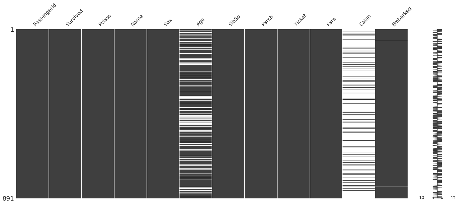
Missing values
Because we have few features we can use the package missingno which allows you to display the completeness of the dataset. It looks there are a lot of missing values for “age” and “cabin” and only 2 for “embarked”.
msno.matrix(TitanicTrain)
Gives this plot:
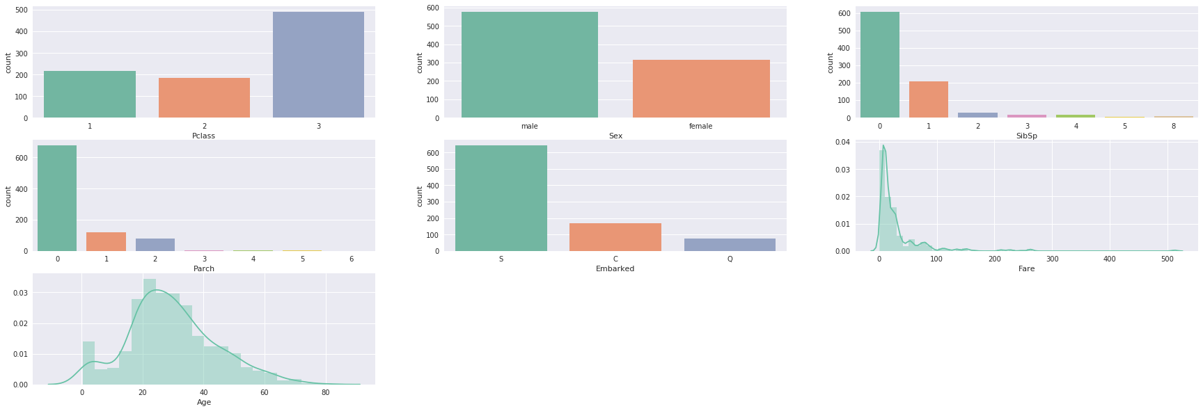
Univariate Analysis
To have a better vision of the data we are going to display our feature with a countplot of seaborn. Show the counts of observations in each categorical bin using bars. The categorical features of our dataset are these are integer and object. We are going to separate our features into two lists: “categ” for the categorical features and “conti” for the continuous features. The “age” and the “fare” are the only two features that we can consider as continuous. In order to plot the distribution of the features with seaborn we are going to use distplot. According to the charts, there are no weird values (superior at 100) for “age” but we can see that the feature “fare” have a large scale and the most of value are between 0 and 100.
categ =  [ 'Pclass', 'Sex', 'SibSp', 'Parch', 'Embarked']
conti = ['Fare', 'Age']

#Distribution
fig = plt.figure(figsize=(30, 10))
for i in range (0,len(categ)):
    fig.add_subplot(3,3,i+1)
    sns.countplot(x=categ[i], data=TitanicTrain);

for col in conti:
    fig.add_subplot(3,3,i + 2)
    sns.distplot(TitanicTrain[col].dropna());
    i += 1

plt.show()
fig.clear()
Gives this plot:
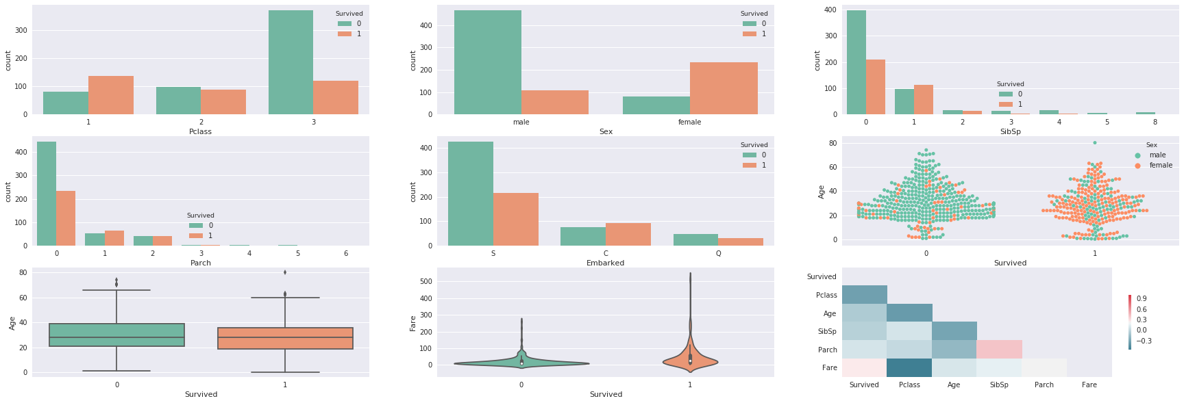
Bivariate Analysis
The next charts show us the repartition of survival (and non-survival) for each features categ and conti. We are going to use others kind of charts to display the relation between ‘survival” and our features. It seems that there are a lot of “female” who have not survived when we take a look at the 6th chart. WIth the boxplot, we can see that there are no outliers in the features “age” (maybe 3-4 observations which are out of the frame but nothing alarming). As concerning the correlation between the features, we can see that the stronger correlation in absolute with “survived” are “fare” and “pclass”. The fact of “fare” and “pclass” have a strong correlation in absolute is consistent and it shows that a priori the people with the upper class spend more money (to have a better place).
fig = plt.figure(figsize=(30, 10))
i = 1
for col in categ:
    if col != 'Survived':
        fig.add_subplot(3,3,i)
        sns.countplot(x=col, data=TitanicTrain,hue='Survived');
        i += 1

# Box plot survived x age
fig.add_subplot(3,3,6)
sns.swarmplot(x="Survived", y="Age", hue="Sex", data=TitanicTrain);
fig.add_subplot(3,3,7)
sns.boxplot(x="Survived", y="Age", data=TitanicTrain)

# fare and Survived
fig.add_subplot(3,3,8)
sns.violinplot(x="Survived", y="Fare", data=TitanicTrain)

# correlations with the new features
corr = TitanicTrain.drop(['PassengerId'], axis=1).corr()
mask = np.zeros_like(corr, dtype=np.bool)
mask[np.triu_indices_from(mask)] = True
cmap = sns.diverging_palette(220, 10, as_cmap=True)
fig.add_subplot(3,3,9)
sns.heatmap(corr, mask=mask, cmap=cmap, cbar_kws={"shrink": .5})
plt.show()
fig.clear()
Gives this plot:
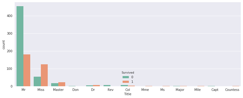
Feature engineering
We going to create one new feature from the dataset. It is possible to create lot of new features with this data. But we are going to exploit the data that we can find through the “title”. I advise you to implement a first model (Quick & Dirty model) before the creation of new features. It is not always interesting to create a new features so you must quantify (with the metrics) if the creation has a positive impact on your model. In this example we start from the assumption that the new feature have a positive impact. We are not sure that the “title” feature give more information than the sex feature.
title = ['Mlle','Mrs', 'Mr', 'Miss','Master','Don','Rev','Dr','Mme','Ms','Major','Col','Capt','Countess']

def ExtractTitle(name):
    tit = 'missing'
    for item in title :
        if item in name:
            tit = item
    if tit == 'missing':
        tit = 'Mr'
    return tit

TitanicTrain["Title"] = TitanicTrain.apply(lambda row: ExtractTitle(row["Name"]),axis=1)
plt.figure(figsize=(13, 5))
fig.add_subplot(2,1,1)
sns.countplot(x='Title', data=TitanicTrain,hue='Survived');
Gives this plot:
Machine Learning
Now we are going to pass at the part of Machine Learning. Within this part we are just tested few models. I will expose you a good way to do a robust cross validation through another tutorial. In this example we will implement a basic sampling (70% train vs 30% test). Yet it is not the better way to implement a robust sampling. Contrary a robust validation this kind of of sampling can bring the overfitting in your model. Keep in mind it is just a “getting started”.
Impute missing value
In the first part we have already seen that there are missing values. In general rules a good imputation is the median (for the numerical features). Yet it is the same thing that the feature engineering: It will be more interesting if you can test different imputations and find the values with the best impact on your metrics. The median is a simple method and you can implement a machine learning method to impute the missing values. For the categorical features we are imputed the missing values by the most frequent values.
# Age
MedianAge = TitanicTrain.Age.median()
TitanicTrain.Age = TitanicTrain.Age.fillna(value=MedianAge)
# Embarked replace NaN with the mode value
ModeEmbarked = TitanicTrain.Embarked.mode()[0]
TitanicTrain.Embarked = TitanicTrain.Embarked.fillna(value=ModeEmbarked)
# Fare have 1 NaN missing value on the Submission dataset
MedianFare = TitanicTrain.Fare.median()
TitanicTrain.Fare = TitanicTrain.Fare.fillna(value=MedianFare)
Encode Categorical features
Another important part of the preprocessing is the processing of categorical features. There are several ways to do that and certain are more suited if there are several categories through the features (Entity Embeddings). In our case we are going to use the function get_dummies which allow you to transform the categorical features in binary features. You can try the function OneHotEncoder of sklearn to do the same thing. In our example there are several values for the features “cabin”, so we have decided to binarize this one in order to use get_dummies. The function get_dummies is not recommended if your categorical features have too many categories also you must investigate on the techniqu of entity embeddings.
# Cabin
TitanicTrain["Cabin"] = TitanicTrain.apply(lambda obs: "No" if pd.isnull(obs['Cabin']) else "Yes", axis=1)
TitanicTrain = pd.get_dummies(TitanicTrain,drop_first=True,columns=['Sex','Title','Cabin','Embarked'])
2.3 Scaling numerical features
The final part of our preprocessing ! The goal of this one is to rescale the numerical features. You can find lot of method through this link http://scikit-learn.org/stable/modules/classes.html#module-sklearn.preprocessing. We are used a simple method for the feature Fare and Age.
scale = StandardScaler().fit(TitanicTrain[['Age', 'Fare']])
TitanicTrain[['Age', 'Fare']] = scale.transform(TitanicTrain[['Age', 'Fare']])
We stop here for the preprocessing. Before the next part it is necessary to create the train and test samples. Like i have already said this kind of sampling is not the best and we will come back on this part through another tutorial entitled “Cross Validation Out Of Bag with Python”.
Target = TitanicTrain.Survived
Features = TitanicTrain.drop(['Survived','Name','Ticket','PassengerId'],axis=1)

# Create training and test sets
X_train, X_test, y_train, y_test = train_test_split(Features, Target, test_size = 0.3, random_state=42)
Target = TitanicTrain.Survived

MlRes= {}
def MlResult(model,score):
    MlRes[model] = score
    print(MlRes)

roc_curve_data = {}
def ConcatRocData(algoname, fpr, tpr, auc):
    data = [fpr, tpr, auc]
    roc_curve_data[algoname] = data
Logistic Regression
The first model that we are going to use is the logistic regression. It is a linear model widespread. Fast, easy to use and easy to understand this model must be part of your toolbox. The fact of being a linear model demands in general rules more preprocessing to have the best results. For our example we have kept just one dataset but keep in mind that a good practice is to work with one dataset for the linear models and another one for the non-linear model.
# Logistic Regression :
logi_reg = LogisticRegression()
# Fit the regressor to the training data
logi_reg.fit(X_train, y_train)
# Predict on the test data: y_pred
y_pred = logi_reg.predict(X_test)
# Score / Metrics
accuracy = logi_reg.score(X_test, y_test)
MlResult('Logistic Regression',accuracy)
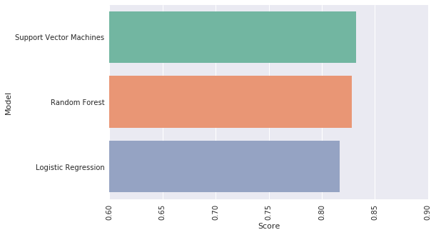
{'Logistic Regression': 0.8283582089552238}
Random Forest
The second model is the Random Forest. For my part i prefer to use Extremely randomized trees (ExtraTreesClassifier in sklearn) which is better than the Random Forest in term of variance. In general rules the extreme version of an algorithm add a layer of penalization or a random layer for a better generalization. You can find here the article on the Extremely randomized trees
# Create a random Forest Classifier instance
rfc = RandomForestClassifier(n_estimators = 100)
# Fit to the training data
rfc.fit(X_train, y_train)
# Predict on the test data: y_pred
y_pred = rfc.predict(X_test)
# Score / Metrics
accuracy = rfc.score(X_test, y_test) # = accuracy
MlResult('Random Forest',accuracy)
{'Logistic Regression': 0.8283582089552238, 'Random Forest': 0.7985074626865671}
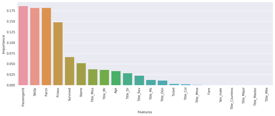
it is possible to display the importances of features with the Random Forest (same thing for Extremely randomized trees). You can take the code and just replace RandomForestClassifier by ExtraTreesClassifier.
#Features importance
def FeaturesImportance(data,model):
    features = data.columns.tolist()
    fi = model.feature_importances_
    sorted_features = {}
    for feature, imp in zip(features, fi):
        sorted_features[feature] = round(imp,3)

    # sort the dictionnary by value
    sorted_features = OrderedDict(sorted(sorted_features.items(),reverse=True, key=lambda t: t[1]))

    #for feature, imp in sorted_features.items():
        #print(feature+" : ",imp)

    dfvi = pd.DataFrame(list(sorted_features.items()), columns=['Features', 'Importance'])
    #dfvi.head()
    plt.figure(figsize=(15, 5))
    sns.barplot(x='Features', y='Importance', data=dfvi);
    plt.xticks(rotation=90)
    plt.show()

#Features importance
FeaturesImportance(TitanicTrain,rfc)
Gives this plot:
Support Vector Machine
Finally I would like to finish with the SVC (Support Vector Classification). The implementation is based on libsvm. “The fit time complexity is more than quadratic with the number of samples which makes it hard to scale to dataset with more than a couple of 10000 samples. The multiclass support is handled according to a one-vs-one scheme.”
svm = SVC(probability=True)
# Fit to the training data
svm.fit(X_train, y_train)
# Predict on the test data: y_pred
y_pred = svm.predict(X_test)

print("Score Support Vector Machines on train data : {}".format(svm.score(X_train, y_train)))
Score Support Vector Machines on train data : 0.8346709470304976
plt.figure(figsize=(8, 5))
sns.barplot(x='Score', y='Model', data=res);
plt.xticks(rotation=90)
plt.xlim([0.6, 0.9])
plt.show()
Conlusion
Like we have said previously it is possible to improve our code with several tasks, for example, it will be good to use a robust cross-validation (to reduce the variance and don’t overfit), it would be nice to reduce the number of features and test others models (Boosting models). As you can see some features have a zero importance. We can also tune parameters for each model with a RandomizedSearchCV.