The purpose of this article is to build a model with Tensorflow. We will see the different steps to do that. The code exposed will allow you to build a regression model, specify the categorical features and build your own activation function with Tensorflow. The data used corresponds to a Kaggle’s competition House Prices: Advanced Regression Techniques.
We will expose three models. The first one will use just the continuous features. For the second one, I will add the categorical features and lastly, I will use a Shallow Neural Network (with just one hidden layer). They are no tuning and we will use DNNRegressor with Relu for all activations functions and the number of units by layer are: [200, 100, 50, 25, 12].
Importation and Devices Available
Before the importation, I prefer to check the devices available. In our example, I have used CPUs. It is always interesting to check if the devices that you are supposed to use are detected. I have already been in the case where I was supposed to use GPUs but the configuration was not done well and the devices detected was not the right. It is problematic when you need a lot of computational power (For example with Speech To Text, Image Recognition and so on…)
from tensorflow.python.client import device_lib
device_lib.list_local_devices()
[name: "/device:CPU:0"
 device_type: "CPU"
 memory_limit: 268435456
 locality {
 }
 incarnation: 2198571128047982842]
Now that I have checked the devices available I will test them with a simple computation. Here we have an example with the computation with the CPU. It is possible to split the computation on your GPUs. Here an example if you have three GPU’s available: ‘with tf.device(‘/gpu:0′):’, ‘with tf.device(‘/gpu:1’): ‘, ‘with tf.device(‘/gpu:2’): ‘ etc…
# Test with a simple computation
import tensorflow as tf

tf.Session()

with tf.device('/cpu:0'):
    a = tf.constant([1.0, 2.0, 3.0, 4.0, 5.0, 6.0], shape=[2, 3])
# If you have gpu you can try this line to compute b with your GPU
#with tf.device('/gpu:0'):
    b = tf.constant([1.0, 2.0, 3.0, 4.0, 5.0, 6.0], shape=[3, 2])
c = tf.matmul(a, b)
# Creates a session with log_device_placement set to True.
sess = tf.Session(config=tf.ConfigProto(log_device_placement=True))

print(sess.run(c))

# Runs the op.
# Log information
options = tf.RunOptions(output_partition_graphs=True)
metadata = tf.RunMetadata()
c_val = sess.run(c, options=options, run_metadata=metadata)

print(metadata.partition_graphs)

sess.close()
[[22. 28.]
 [49. 64.]]
[node {
  name: "MatMul"
  op: "Const"
  device: "/job:localhost/replica:0/task:0/device:CPU:0"
  attr {
    key: "dtype"
    value {
      type: DT_FLOAT
    }
  }
  attr {
    key: "value"
    value {
      tensor {
        dtype: DT_FLOAT
        tensor_shape {
          dim {
            size: 2
          }
          dim {
            size: 2
          }
        }
        tensor_content: "\000\000\260A\000\000\340A\000\000DB\000\000\200B"
      }
    }
  }
}
node {
  name: "_retval_MatMul_0_0"
  op: "_Retval"
  input: "MatMul"
  device: "/job:localhost/replica:0/task:0/device:CPU:0"
  attr {
    key: "T"
    value {
      type: DT_FLOAT
    }
  }
  attr {
    key: "index"
    value {
      i: 0
    }
  }
}
library {
}
versions {
  producer: 26
}
]
So now that we are sure that the devices are detected well we can start to work with the data. In this tutorial our <a href="http://train“>train data is composed to 1460 rows with 81 features. 38 continuous features and 43 categorical features. As exposed in the introduction we will use only the continuous features to build our first model. You can find the test data here.
Here the objective is to predict the House Prices. We have a problem of regression. So our first data will contain 37 features to explain the ‘SalePrice’. We can see the list of features that we will use to build our first model.
from __future__ import absolute_import
from __future__ import division
from __future__ import print_function

import itertools

import pandas as pd
import numpy as np
import matplotlib.pyplot as plt
from pylab import rcParams
import matplotlib

from sklearn.model_selection import train_test_split
from sklearn.preprocessing import MinMaxScaler

tf.logging.set_verbosity(tf.logging.INFO)
sess = tf.InteractiveSession()

train = pd.read_csv('../input/train.csv')
print('Shape of the train data with all features:', train.shape)
train = train.select_dtypes(exclude=['object'])
print("")
print('Shape of the train data with numerical features:', train.shape)
train.drop('Id',axis = 1, inplace = True)
train.fillna(0,inplace=True)

test = pd.read_csv('../input/test.csv')
test = test.select_dtypes(exclude=['object'])
ID = test.Id
test.fillna(0,inplace=True)
test.drop('Id',axis = 1, inplace = True)

print("")
print("List of features contained our dataset:",list(train.columns))
Shape of the train data with all features: (1460, 81)

The shape of the train data with numerical features: (1460, 38)

List of features contained our dataset: ['MSSubClass', 'LotFrontage', 'LotArea', 'OverallQual', 'OverallCond', 'YearBuilt', 'YearRemodAdd', 'MasVnrArea', 'BsmtFinSF1', 'BsmtFinSF2', 'BsmtUnfSF', 'TotalBsmtSF', '1stFlrSF', '2ndFlrSF', 'LowQualFinSF', 'GrLivArea', 'BsmtFullBath', 'BsmtHalfBath', 'FullBath', 'HalfBath', 'BedroomAbvGr', 'KitchenAbvGr', 'TotRmsAbvGrd', 'Fireplaces', 'GarageYrBlt', 'GarageCars', 'GarageArea', 'WoodDeckSF', 'OpenPorchSF', 'EnclosedPorch', '3SsnPorch', 'ScreenPorch', 'PoolArea', 'MiscVal', 'MoSold', 'YrSold', 'SalePrice']
Outliers
In this part, we will isolate the outliers with an IsolationForest (http://scikit-learn.org/stable/modules/generated/sklearn.ensemble.IsolationForest.html). I tried with and without this step and I had a better performance removing these rows. I haven’t analyzed the test set but I suppose that our train set looks like more at our data test without these outliers.
from sklearn.ensemble import IsolationForest

clf = IsolationForest(max_samples = 100, random_state = 42)
clf.fit(train)
y_noano = clf.predict(train)
y_noano = pd.DataFrame(y_noano, columns = ['Top'])
y_noano[y_noano['Top'] == 1].index.values

train = train.iloc[y_noano[y_noano['Top'] == 1].index.values]
train.reset_index(drop = True, inplace = True)
print("Number of Outliers:", y_noano[y_noano['Top'] == -1].shape[0])
print("Number of rows without outliers:", train.shape[0])
Number of Outliers: 146
Number of rows without outliers: 1314
Preprocessing
The first preprocessing of our data will be to rescale our features and we will use the function MinMaxScaler of Scikit-learn.
import warnings
warnings.filterwarnings('ignore')

col_train = list(train.columns)
col_train_bis = list(train.columns)

col_train_bis.remove('SalePrice')

mat_train = np.matrix(train)
mat_test  = np.matrix(test)
mat_new = np.matrix(train.drop('SalePrice',axis = 1))
mat_y = np.array(train.SalePrice).reshape((1314,1))

prepro_y = MinMaxScaler()
prepro_y.fit(mat_y)

prepro = MinMaxScaler()
prepro.fit(mat_train)

prepro_test = MinMaxScaler()
prepro_test.fit(mat_new)

train = pd.DataFrame(prepro.transform(mat_train),columns = col_train)
test  = pd.DataFrame(prepro_test.transform(mat_test),columns = col_train_bis)
To use Tensorflow we need to transform our data (features) in a special format. As a reminder, we have just the continuous features. So the first function used is: tf.contrib.layers.real_valued_column. The others cells allowed to us to create a train set and test set with our training dataset. The sampling is not the most relevant but it is not the goal of this article. So be careful! The sample 67-33 is not the rule!
# List of features
COLUMNS = col_train
FEATURES = col_train_bis
LABEL = "SalePrice"

# Columns for tensorflow
feature_cols = [tf.contrib.layers.real_valued_column(k) for k in FEATURES]

# Training set and Prediction set with the features to predict
training_set = train[COLUMNS]
prediction_set = train.SalePrice

# Train and Test
x_train, x_test, y_train, y_test = train_test_split(training_set[FEATURES] , prediction_set, test_size=0.33, random_state=42)
y_train = pd.DataFrame(y_train, columns = [LABEL])
training_set = pd.DataFrame(x_train, columns = FEATURES).merge(y_train, left_index = True, right_index = True)

# Training for submission
training_sub = training_set[col_train]

# Same thing but for the test set
y_test = pd.DataFrame(y_test, columns = [LABEL])
testing_set = pd.DataFrame(x_test, columns = FEATURES).merge(y_test, left_index = True, right_index = True)
Our data is ready to build our first model with Tensorflow!
Deep Neural Network for continuous features
With tf.contrib.learn it is very easy to implement a Deep Neural Network. In our first example, we will have 5 hidden layers with respect 200, 100, 50, 25 and 12 units and the function of activation will be Relu. The optimizer used in our case is an Adagrad optimizer (by default).
# Model
tf.logging.set_verbosity(tf.logging.ERROR)
regressor = tf.contrib.learn.DNNRegressor(feature_columns=feature_cols,
                                          activation_fn = tf.nn.relu, hidden_units=[200, 100, 50, 25, 12])

# Reset the index of training
training_set.reset_index(drop = True, inplace =True)
def input_fn(data_set, pred = False):

    if pred == False:

        feature_cols = {k: tf.constant(data_set[k].values) for k in FEATURES}
        labels = tf.constant(data_set[LABEL].values)

        return feature_cols, labels

    if pred == True:
        feature_cols = {k: tf.constant(data_set[k].values) for k in FEATURES}

        return feature_cols

# Deep Neural Network Regressor with the training set which contain the data split by train test split
regressor.fit(input_fn=lambda: input_fn(training_set), steps=2000)

# Evaluation on the test set created by train_test_split
ev = regressor.evaluate(input_fn=lambda: input_fn(testing_set), steps=1)

# Display the score on the testing set
loss_score1 = ev["loss"]
print("Final Loss on the testing set: {0:f}".format(loss_score1))
Final Loss on the testing set: 0.002229
The model is built ! Now we are going to see how can we use it to compute the predictions.
# Predictions
y = regressor.predict(input_fn=lambda: input_fn(testing_set))
predictions = list(itertools.islice(y, testing_set.shape[0]))
Data Preprocessed: done! Outliers excluded: done! Model built: done! Next step: Used our model to make the predictions with the dataset Test. And add one graphic to see the difference between the reality and the predictions.
predictions = pd.DataFrame(prepro_y.inverse_transform(np.array(predictions).reshape(434,1)),columns = ['Prediction'])
reality = pd.DataFrame(prepro.inverse_transform(testing_set), columns = [COLUMNS]).SalePrice
matplotlib.rc('xtick', labelsize=30)
matplotlib.rc('ytick', labelsize=30)

fig, ax = plt.subplots(figsize=(50, 40))

plt.style.use('ggplot')
plt.plot(predictions.values, reality.values, 'ro')
plt.xlabel('Predictions', fontsize = 30)
plt.ylabel('Reality', fontsize = 30)
plt.title('Predictions x Reality on dataset Test', fontsize = 30)
ax.plot([reality.min(), reality.max()], [reality.min(), reality.max()], 'k--', lw=4)
plt.show()
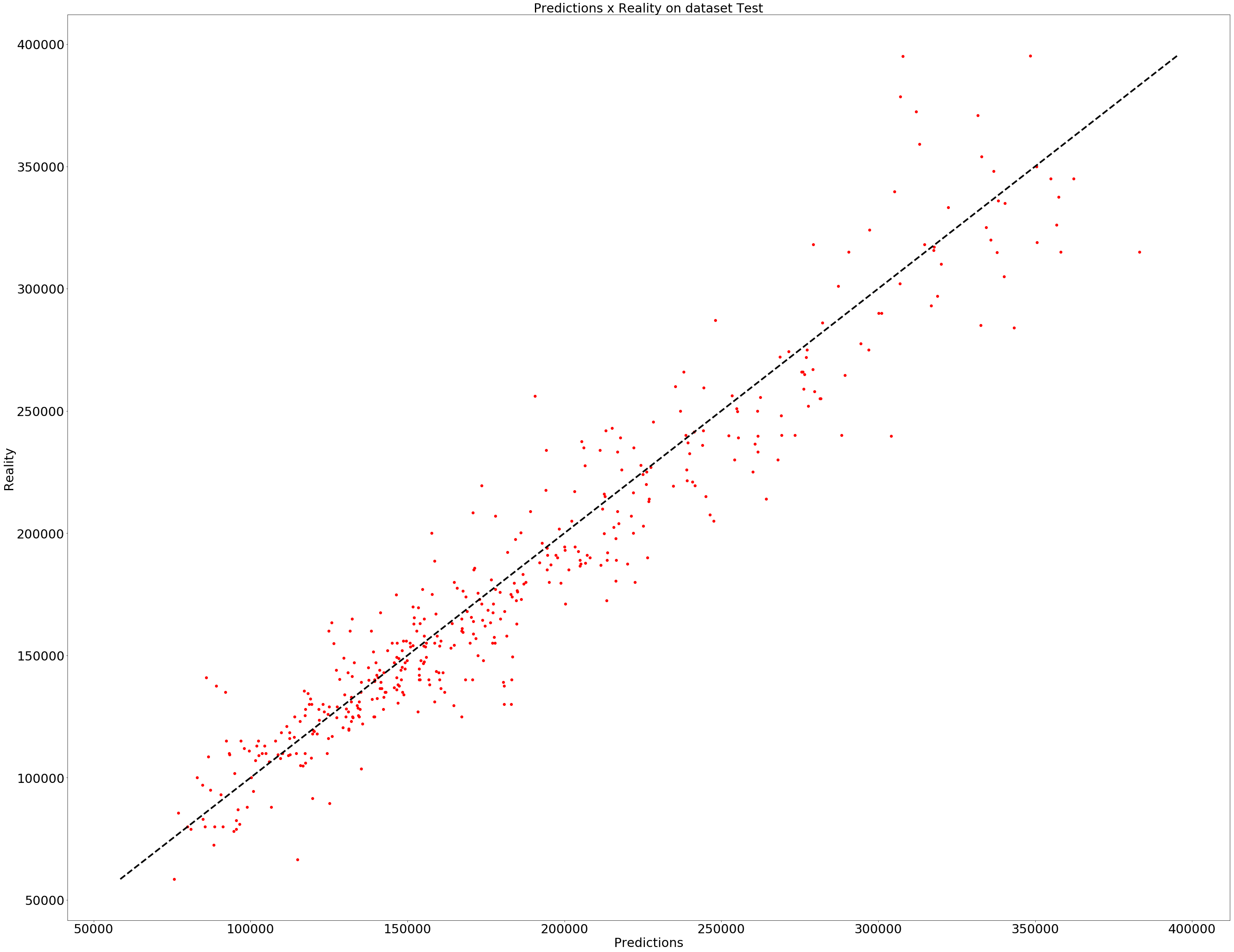
It seems not bad!
Create your own activation function
In our first model we have used the activation function Relu. Now we are going to use our own activation function. It is possible that the function leaky relu is already coded through Tensorflow. But you could use this code to implement your own activation function. As a reminder, Relu is Max(x,0) and Leaky Relu is the function Max(x, delta*x). In our case, we can take delta = 0.01
def leaky_relu(x):
    return tf.nn.relu(x) - 0.01 * tf.nn.relu(-x)

# Model
regressor = tf.contrib.learn.DNNRegressor(feature_columns=feature_cols,
                                          activation_fn = leaky_relu, hidden_units=[200, 100, 50, 25, 12])

# Deep Neural Network Regressor with the training set which contain the data split by train test split
regressor.fit(input_fn=lambda: input_fn(training_set), steps=2000)

# Evaluation on the test set created by train_test_split
ev = regressor.evaluate(input_fn=lambda: input_fn(testing_set), steps=1)

# Display the score on the testing set
loss_score2 = ev["loss"]
print("Final Loss on the testing set with Leaky Relu: {0:f}".format(loss_score2))

# Predictions
y_predict = regressor.predict(input_fn=lambda: input_fn(test, pred = True))
Final Loss on the testing set with Leaky Relu: 0.002556
It is not very complicated! Just before changing of parts, we are going to add another model with the activation function Elu.
# Model
regressor = tf.contrib.learn.DNNRegressor(feature_columns=feature_cols,
                                          activation_fn = tf.nn.elu, hidden_units=[200, 100, 50, 25, 12])

# Deep Neural Network Regressor with the training set which contain the data split by train test split
regressor.fit(input_fn=lambda: input_fn(training_set), steps=2000)

# Evaluation on the test set created by train_test_split
ev = regressor.evaluate(input_fn=lambda: input_fn(testing_set), steps=1)

loss_score3 = ev["loss"]
print("Final Loss on the testing set with Elu: {0:f}".format(loss_score3))

# Predictions
y_predict = regressor.predict(input_fn=lambda: input_fn(test, pred = True))
Final Loss on the testing set with Elu: 0.002447
So we have three models with three different activation functions. But we built our models just with the continuous features. Now we see how do build another model by adding a categorical feature. The following part will show how we can use the categorical features with Tensorflow.
Deep Neural Network for continuous and categorical features
For this part, I repeat the same functions that you can find previously by adding a categorical feature.
# Import and split
train = pd.read_csv('../input/train.csv')
train.drop('Id',axis = 1, inplace = True)
train_numerical = train.select_dtypes(exclude=['object'])
train_numerical.fillna(0,inplace = True)
train_categoric = train.select_dtypes(include=['object'])
train_categoric.fillna('NONE',inplace = True)
train = train_numerical.merge(train_categoric, left_index = True, right_index = True)

test = pd.read_csv('../input/test.csv')
ID = test.Id
test.drop('Id',axis = 1, inplace = True)
test_numerical = test.select_dtypes(exclude=['object'])
test_numerical.fillna(0,inplace = True)
test_categoric = test.select_dtypes(include=['object'])
test_categoric.fillna('NONE',inplace = True)
test = test_numerical.merge(test_categoric, left_index = True, right_index = True)
# Removie the outliers
from sklearn.ensemble import IsolationForest

clf = IsolationForest(max_samples = 100, random_state = 42)
clf.fit(train_numerical)
y_noano = clf.predict(train_numerical)
y_noano = pd.DataFrame(y_noano, columns = ['Top'])
y_noano[y_noano['Top'] == 1].index.values

train_numerical = train_numerical.iloc[y_noano[y_noano['Top'] == 1].index.values]
train_numerical.reset_index(drop = True, inplace = True)

train_categoric = train_categoric.iloc[y_noano[y_noano['Top'] == 1].index.values]
train_categoric.reset_index(drop = True, inplace = True)

train = train.iloc[y_noano[y_noano['Top'] == 1].index.values]
train.reset_index(drop = True, inplace = True)
col_train_num = list(train_numerical.columns)
col_train_num_bis = list(train_numerical.columns)

col_train_cat = list(train_categoric.columns)

col_train_num_bis.remove('SalePrice')

mat_train = np.matrix(train_numerical)
mat_test  = np.matrix(test_numerical)
mat_new = np.matrix(train_numerical.drop('SalePrice',axis = 1))
mat_y = np.array(train.SalePrice)

prepro_y = MinMaxScaler()
prepro_y.fit(mat_y.reshape(1314,1))

prepro = MinMaxScaler()
prepro.fit(mat_train)

prepro_test = MinMaxScaler()
prepro_test.fit(mat_new)

train_num_scale = pd.DataFrame(prepro.transform(mat_train),columns = col_train)
test_num_scale  = pd.DataFrame(prepro_test.transform(mat_test),columns = col_train_bis)
train[col_train_num] = pd.DataFrame(prepro.transform(mat_train),columns = col_train_num)
test[col_train_num_bis]  = test_num_scale
The changements start with the following code. It is possible to use others functions to prepare your categorical data.
# List of features
COLUMNS = col_train_num
FEATURES = col_train_num_bis
LABEL = "SalePrice"

FEATURES_CAT = col_train_cat

engineered_features = []

for continuous_feature in FEATURES:
    engineered_features.append(
        tf.contrib.layers.real_valued_column(continuous_feature))

for categorical_feature in FEATURES_CAT:
    sparse_column = tf.contrib.layers.sparse_column_with_hash_bucket(
        categorical_feature, hash_bucket_size=1000)

    engineered_features.append(tf.contrib.layers.embedding_column(sparse_id_column=sparse_column, dimension=16,combiner="sum"))

# Training set and Prediction set with the features to predict
training_set = train[FEATURES + FEATURES_CAT]
prediction_set = train.SalePrice

# Train and Test
x_train, x_test, y_train, y_test = train_test_split(training_set[FEATURES + FEATURES_CAT] ,
                                                    prediction_set, test_size=0.33, random_state=42)
y_train = pd.DataFrame(y_train, columns = [LABEL])
training_set = pd.DataFrame(x_train, columns = FEATURES + FEATURES_CAT).merge(y_train, left_index = True, right_index = True)

# Training for submission
training_sub = training_set[FEATURES + FEATURES_CAT]
testing_sub = test[FEATURES + FEATURES_CAT]

# Same thing but for the test set
y_test = pd.DataFrame(y_test, columns = [LABEL])
testing_set = pd.DataFrame(x_test, columns = FEATURES + FEATURES_CAT).merge(y_test, left_index = True, right_index = True)
training_set[FEATURES_CAT] = training_set[FEATURES_CAT].applymap(str)
testing_set[FEATURES_CAT] = testing_set[FEATURES_CAT].applymap(str)

def input_fn_new(data_set, training = True):
    continuous_cols = {k: tf.constant(data_set[k].values) for k in FEATURES}

    categorical_cols = {k: tf.SparseTensor(
        indices=[[i, 0] for i in range(data_set[k].size)], values = data_set[k].values, dense_shape = [data_set[k].size, 1]) for k in FEATURES_CAT}

    # Merges the two dictionaries into one.
    feature_cols = dict(list(continuous_cols.items()) + list(categorical_cols.items()))

    if training == True:
        # Converts the label column into a constant Tensor.
        label = tf.constant(data_set[LABEL].values)

        # Returns the feature columns and the label.
        return feature_cols, label

    return feature_cols

# Model
regressor = tf.contrib.learn.DNNRegressor(feature_columns = engineered_features,
                                          activation_fn = tf.nn.relu, hidden_units=[200, 100, 50, 25, 12])

categorical_cols = {k: tf.SparseTensor(indices=[[i, 0] for i in range(training_set[k].size)], values = training_set[k].values, dense_shape = [training_set[k].size, 1]) for k in FEATURES_CAT}

# Deep Neural Network Regressor with the training set which contain the data split by train test split
regressor.fit(input_fn = lambda: input_fn_new(training_set) , steps=2000)

ev = regressor.evaluate(input_fn=lambda: input_fn_new(testing_set, training = True), steps=1)
loss_score4 = ev["loss"]

print("Final Loss on the testing set: {0:f}".format(loss_score4))

# Predictions
y = regressor.predict(input_fn=lambda: input_fn_new(testing_set))
predictions = list(itertools.islice(y, testing_set.shape[0]))
predictions = pd.DataFrame(prepro_y.inverse_transform(np.array(predictions).reshape(434,1)))
Final Loss on the testing set: 0.002189
Shallow Network
For this part, we will explore the architecture with just one Hidden Layer with several units. The question is: How many units do you need to have a good score? We will try with 1000 units with the activation function Relu. You can find more informations here on the difference between the shallow and the deep neural network.
# Model
regressor = tf.contrib.learn.DNNRegressor(feature_columns = engineered_features,
                                          activation_fn = tf.nn.relu, hidden_units=[1000])

# Deep Neural Network Regressor with the training set which contain the data split by train test split
regressor.fit(input_fn = lambda: input_fn_new(training_set) , steps=2000)

ev = regressor.evaluate(input_fn=lambda: input_fn_new(testing_set, training = True), steps=1)
loss_score5 = ev["loss"]

print("Final Loss on the testing set: {0:f}".format(loss_score5))

y_predict = regressor.predict(input_fn=lambda: input_fn_new(testing_sub, training = False))
Final Loss on the testing set: 0.001728
Conclusion
list_score = [loss_score1, loss_score2, loss_score3, loss_score4,loss_score5]
list_model = ['Relu_cont', 'LRelu_cont', 'Elu_cont', 'Relu_cont_categ','Shallow_1ku']
import matplotlib.pyplot as plt; plt.rcdefaults()

plt.style.use('ggplot')
objects = list_model
y_pos = np.arange(len(objects))
performance = list_score

plt.barh(y_pos, performance, align='center', alpha=0.9)
plt.yticks(y_pos, objects)
plt.xlabel('Loss ')
plt.title('Model compared without hypertuning')
plt.show()
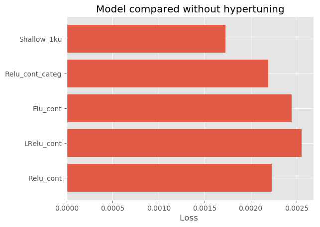
So, I hope that this small introduction will be useful! With this code, you can build a regression model with Tensorflow with continuous and categorical features plus add a new activation function. The results are not significant! In my case, we can see that the Shallow Neural Network are better than the others architecture but there were no optimizations and the sampling was basic. It will be interesting to compare the time between each architecture.