Twitter Analysis with Python

Twitter is a good ressource to collect data. We can find a few libraries (R or Python) which allow you to build your own dataset with the data generated by Twitter. This tutorial is focus on the preparation of the data and no on the collect. Throughout this analysis we are going to see how to work with the twitter’s data. If You want to play with the same data you can download it here.

Importation & cleaning

In this section we are going to focus on the most important part of the analysis. In general rule the tweet are composed by several strings that we have to clean before working correctly with the data. I have separated the importation of package into three parts. As usual Numpy and Pandas are part of our toolbox.

For the visualisation we use Seaborn, Matplotlib, Basemap and word_cloud. In order to clean our data (text) and to do the sentiment analysis the most common library is NLTK. NLTK is a leading platform Python programs to work with human language data. It exists another Natural Language Toolkit (Gensim) but in our case it is not necessary to use it.

import numpy as np
import pandas as pd
import re
import warnings

#Visualisation
import matplotlib.pyplot as plt
import matplotlib
import seaborn as sns
from IPython.display import display
from mpl_toolkits.basemap import Basemap
from wordcloud import WordCloud, STOPWORDS

#nltk
from nltk.stem import WordNetLemmatizer
from nltk.sentiment.vader import SentimentIntensityAnalyzer
from nltk.sentiment.util import *
from nltk import tokenize

matplotlib.style.use('ggplot')
pd.options.mode.chained_assignment = None
warnings.filterwarnings("ignore")

%matplotlib inline

tweets = pd.read_csv('../input/tweets_all.csv', encoding = "ISO-8859-1")

The data with which are going to work is a list of tweets with the hashtag #goodmorning. Our dataset is composed by 43 columns. But only a few columns will be concerned by our analysis. In this analysis we are kept the column “text” which contains the text of the tweet, the column “country” which contains the user’s country, the column “source” which contains the user’s device (and others information) and finally the columns “place_lon”, “place_lat” which contains the longitude and the latitude of the user.

Here an example of the first column whereby we are going to start.

tweets['text'][1]
'@DinaPugliese Good morning Dina :) Have a terrific hump day! :) Little snowy in Cochrane today. https://t.co/P3j1dtUs6y'

You can see that in the first tweet we can find an URL, punctuations and a username of one tweetos (preceded by @). Before the data visualisation or the sentiment analysis it is necessary to clean the data. Delete the punctuations, the URLs, put the test in a lower case, extract the username for examples. It is possible to add more steps but in our case it won’t be useful.

For the first step we are going to extract the username through the tweets (preceded by @ or by RT @). We keep this information in the column “tweetos”.

#Preprocessing del RT @blablabla:
tweets['tweetos'] = '' 

#add tweetos first part
for i in range(len(tweets['text'])):
    try:
        tweets['tweetos'][i] = tweets['text'].str.split(' ')[i][0]
    except AttributeError:    
        tweets['tweetos'][i] = 'other'

#Preprocessing tweetos. select tweetos contains 'RT @'
for i in range(len(tweets['text'])):
    if tweets['tweetos'].str.contains('@')[i]  == False:
        tweets['tweetos'][i] = 'other'
        
# remove URLs, RTs, and twitter handles
for i in range(len(tweets['text'])):
    tweets['text'][i] = " ".join([word for word in tweets['text'][i].split()
                                if 'http' not in word and '@' not in word and '<' not in word])


tweets['text'][1]
'Good morning Dina :) Have a terrific hump day! :) Little snowy in Cochrane today.'

We can see that the first step of the cleaning it well done ! The username and the URL are deleted correctly. Now we are going to delete certains punctuations, put the text in lower case and delete the double space with the function apply.

tweets['text'] = tweets['text'].apply(lambda x: re.sub('[!@#$:).;,?&]', '', x.lower()))
tweets['text'] = tweets['text'].apply(lambda x: re.sub('  ', ' ', x))
tweets['text'][1]
'good morning dina have a terrific hump day little snowy in cochrane today'

All steps are completed! We have the tweets cleaned. Now we are going to do the second part.

Visualisation with WordCloud

In this part, we are going to focus on the kind of data visualisation “word cloud”. It always interesting to do this kind of viz in order to have a global vision when you have text data. The visualisation are going to do with the column “text” and “country”.

def wordcloud(tweets,col):
    stopwords = set(STOPWORDS)
    wordcloud = WordCloud(background_color="white",stopwords=stopwords,random_state = 2016).generate(" ".join([i for i in tweets[col]]))
    plt.figure( figsize=(20,10), facecolor='k')
    plt.imshow(wordcloud)
    plt.axis("off")
    plt.title("Good Morning Datascience+")
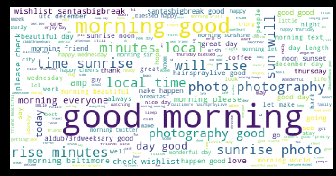
wordcloud(tweets,'text')  

tweets['country'] = tweets['country'].apply(lambda x: x.lower())
tweets['country'].replace('states united','united states',inplace=True)
tweets['country'].replace('united states','usa',inplace=True)
tweets['country'].replace('united Kingdom','uk',inplace=True)
tweets['country'].replace('republic philippines','philippines republic',inplace=True)
wordcloud(tweets, 'country')  

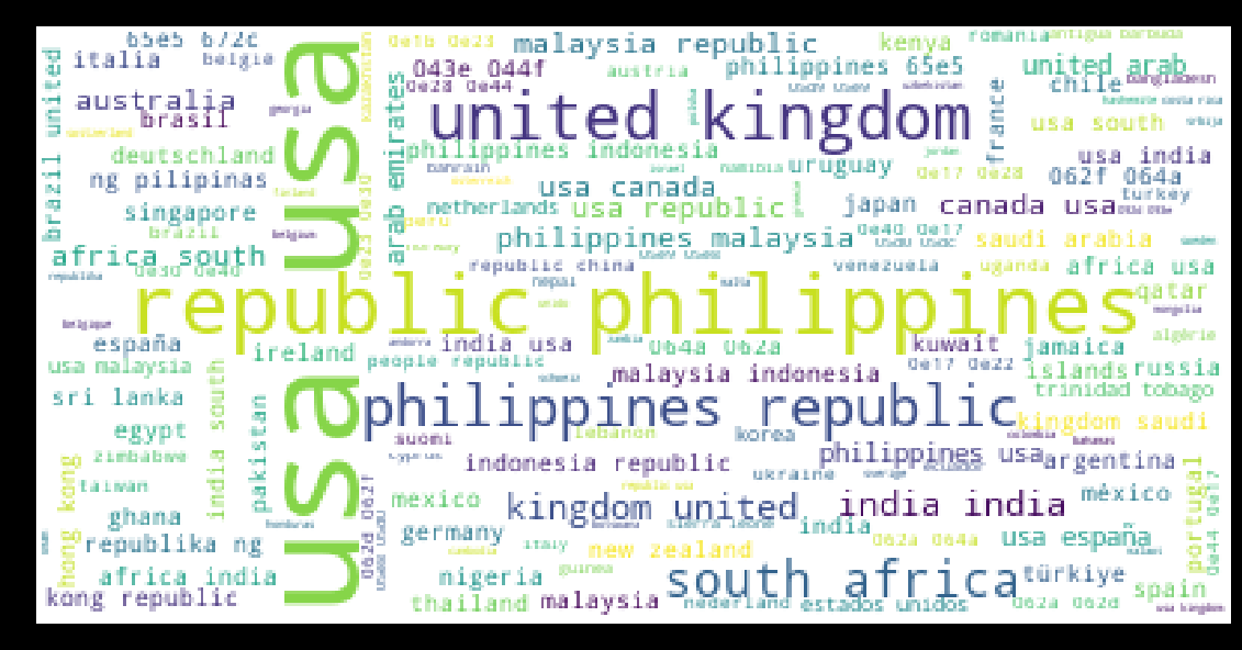
The most of tweets contain the words “good morning” (it is not surprising because the tweets are selected with the hashtag #goodmorning), “photography”, “good day”, “sunrise” and so on… We can already think that the sentiment analysis will be positive in the most of cases. Regarding the information on the countries we can see that the most of tweets are sent from United States, Philippines, United Kingdom and South Africa.

Tweet’s sources

In this third part we are going to check the source of the tweets. And by the “source” I mean the device and the location. As usual the first step is the cleaning. The kind of device is situated at the end in the column “source”. With the following example we can see that the device is just before “/a>”.

tweets['source'][2]
'Twitter for Android'

tweets['source_new'] = ''

for i in range(len(tweets['source'])):
    m = re.search('(?)(.*)', tweets['source'][i])
    try:
        tweets['source_new'][i]=m.group(0)
    except AttributeError:
        tweets['source_new'][i]=tweets['source'][i]
        
tweets['source_new'] = tweets['source_new'].str.replace('', ' ', case=False)

We are going to create another column which will contain the source cleaned. Here the top five of the column “source_new”.

tweets['source_new'].head()
0              Instagram 
1    Twitter for Android 
2    Twitter for Android 
3    Twitter for Android 
4     Twitter Web Client 
Name: source_new, dtype: object

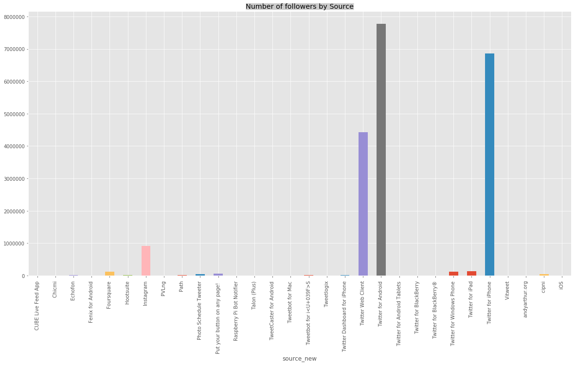
What we interest us is the number of a tweet by source. With the following lines, we are going to compute this indicator.

tweets_by_type = tweets.groupby(['source_new'])['followers_count'].sum()
plt.title('Number of followers by Source', bbox={'facecolor':'0.8', 'pad':0})
tweets_by_type.transpose().plot(kind='bar',figsize=(20, 10))

tweets['source_new2'] = ''

for i in range(len(tweets['source_new'])):
    if tweets['source_new'][i] not in ['Twitter for Android ','Instagram ','Twitter Web Client ','Twitter for iPhone ']:
        tweets['source_new2'][i] = 'Others'
    else:
        tweets['source_new2'][i] = tweets['source_new'][i] 

tweets_by_type2 = tweets.groupby(['source_new2'])['followers_count'].sum()
tweets_by_type2.rename("",inplace=True)
explode = (1, 0, 0, 0, 0)
tweets_by_type2.transpose().plot(kind='pie',figsize=(20, 15),autopct='%1.1f%%',shadow=True,explode=explode)
plt.legend(bbox_to_anchor=(1, 1), loc=6, borderaxespad=0.)
plt.title('Number of followers by Source bis', bbox={'facecolor':'0.8', 'pad':5})

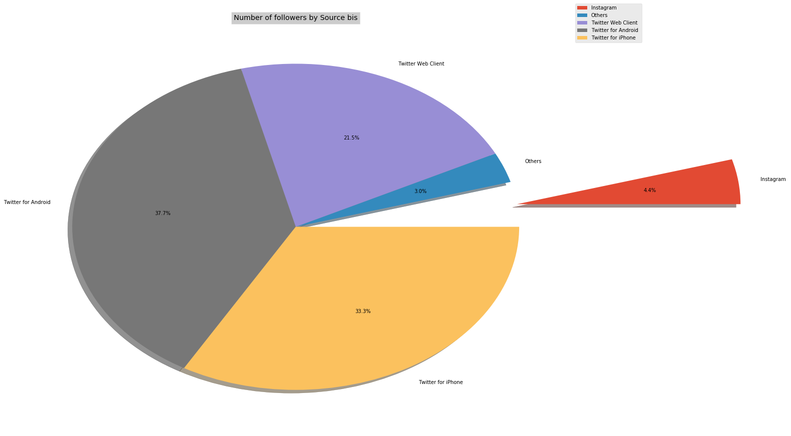
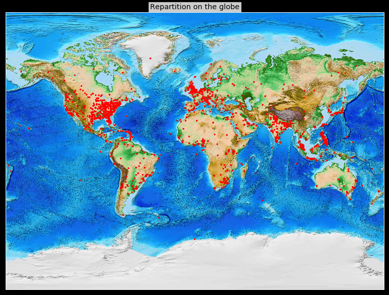
These charts show us that the most important part of the tweet is sent through iPhone, Android, and Webclient. And only 7% by Instagram and other devices. Now we are going to interest in the information of the localization: longitude and latitude. To display this information through a visualization we are going to use “Basemap”. Each red point corresponds to a location.

plt.figure( figsize=(20,10), facecolor='k')
m = Basemap(projection='mill',resolution=None,llcrnrlat=-90,urcrnrlat=90,llcrnrlon=-180,urcrnrlon=180)
m.etopo()
xpt,ypt = m(np.array(tweets['place_lon']),np.array(tweets['place_lat']))
lon,lat = m(xpt,ypt,inverse=True)
m.plot(xpt,ypt,'ro',markersize=np.sqrt(5)) 
plt.title('Repartition on the globe', bbox={'facecolor':'0.8', 'pad':3})
plt.show()

Sentiment analysis

Throughout last part, we are going to do an sentiment analysis. The objective is to class by type the tweets. We are going to distinguish 3 kinds of tweets according to their polarity score. We will have the positive tweets, the neutral tweets, and the negative tweets.

tweets['text_lem'] = [''.join([WordNetLemmatizer().lemmatize(re.sub('[^A-Za-z]', ' ', line)) for line in lists]).strip() for lists in tweets['text']]       
vectorizer = TfidfVectorizer(max_df=0.5,max_features=10000,min_df=10,stop_words='english',use_idf=True)
X = vectorizer.fit_transform(tweets['text_lem'].str.upper())
sid = SentimentIntensityAnalyzer()
tweets['sentiment_compound_polarity']=tweets.text_lem.apply(lambda x:sid.polarity_scores(x)['compound'])
tweets['sentiment_neutral']=tweets.text_lem.apply(lambda x:sid.polarity_scores(x)['neu'])
tweets['sentiment_negative']=tweets.text_lem.apply(lambda x:sid.polarity_scores(x)['neg'])
tweets['sentiment_pos']=tweets.text_lem.apply(lambda x:sid.polarity_scores(x)['pos'])
tweets['sentiment_type']=''
tweets.loc[tweets.sentiment_compound_polarity>0,'sentiment_type']='POSITIVE'
tweets.loc[tweets.sentiment_compound_polarity==0,'sentiment_type']='NEUTRAL'
tweets.loc[tweets.sentiment_compound_polarity<0,'sentiment_type']='NEGATIVE'

tweets_sentiment = tweets.groupby(['sentiment_type'])['sentiment_neutral'].count()
tweets_sentiment.rename("",inplace=True)
explode = (1, 0, 0)
plt.subplot(221)
tweets_sentiment.transpose().plot(kind='barh',figsize=(20, 20))
plt.title('Sentiment Analysis 1', bbox={'facecolor':'0.8', 'pad':0})
plt.subplot(222)
tweets_sentiment.plot(kind='pie',figsize=(20, 20),autopct='%1.1f%%',shadow=True,explode=explode)
plt.legend(bbox_to_anchor=(1, 1), loc=3, borderaxespad=0.)
plt.title('Sentiment Analysis 2', bbox={'facecolor':'0.8', 'pad':0})
plt.show()

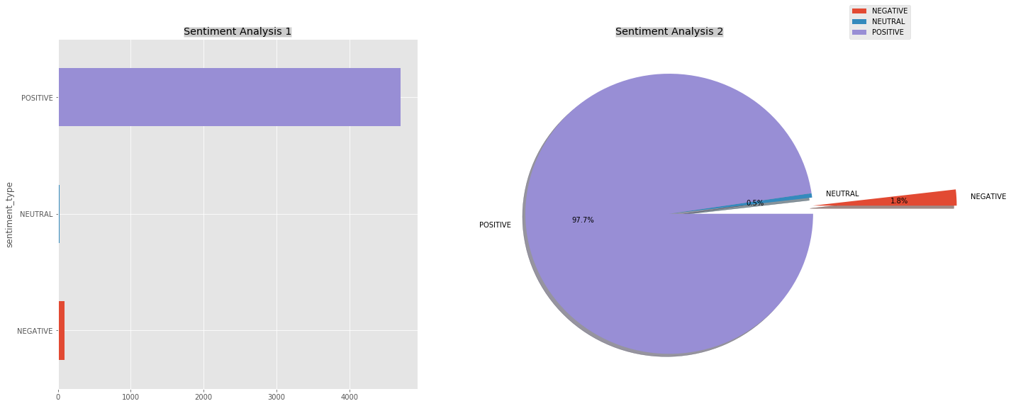
tweets[tweets.sentiment_type == 'NEGATIVE'].text.reset_index(drop = True)[0:5]
0    good morning it's time for pastries almond and...
1                                   good morning bitch
2    not a good look when you take a study break to...
3    good morning niece/ it's been awhile- miss you...
4                   good morning from hell that is all
Name: text, dtype: object

You can see the non-comprehensive list of tweets which are considered negative. It will be interested to identify the words which contribute to put a negative sentiment and why not compared NLTK versus Gensim on the sentiment analysis. In general rule, the data that you can download from Twitter has the same structure. So you can easily create your own dataset and run the code expose within this tutorial (with a few updates).