This tutorial introduces the processing of a huge dataset in python. It allows you to work with a big quantity of data with your own laptop. With this method, you could use the aggregation functions on a dataset that you cannot import in a DataFrame.
In our example, the machine has 32 cores with 17GB of Ram. About the data the file is named user_log.csv, the number of rows of the dataset is 400 Million (6.7 GB zipped) and it corresponds at the daily user logs describing listening behaviors of a user.
About the features:
- – msno: user id
– date: format %Y%m%d
– num_25: # of songs played less than 25% of the song length
– num_50: # of songs played between 25% to 50% of the song length
– num_75: # of songs played between 50% to 75% of the song length
– num_985: # of songs played between 75% to 98.5% of the song length
– num_100: # of songs played over 98.5% of the song length
– num_unq: # of unique songs played
– total_secs: total seconds played
Our tutorial is composed by two parts. The first parts will be a focus on the data aggregation. It is not possible to import all data within a data frame and then to do the aggregation.
You could find several rows by users in the dataset and you are going to show how aggregate our 400 Million rows to have a dataset aggregated with one row by users. In the second part, we are going to continue the processing but this time in order to optimize the memory usage with a few transformations.
# Load the required packages
import time
import psutil
import numpy as np
import pandas as pd
import multiprocessing as mp

# Check the number of cores and memory usage
num_cores = mp.cpu_count()
print("This kernel has ",num_cores,"cores and you can find the information regarding the memory usage:",psutil.virtual_memory())
This kernel has  32 cores and you can find the information regarding the memory usage: svmem(total=121466597376, available=91923750912, percent=24.3, used=27252092928, free=63477522432, active=46262022144, inactive=9810317312, buffers=1972326400, cached=28764655616, shared=1120292864)
The package multiprocessing shows you the number of core of your machine whereas the package psutil shows different information on the memory of your machine. The only ones packages that we need to do our processing is pandas and numpy. time will be use just to display the duration for each iteration.
Aggregation
The aggregation functions selected are min, max and count for the feature “date” and sum for the features “num_25”, “num_50”, “num_75”, “num_985”, “num_100”, “num_unq” and “totalc_secs”. Therefore for each customers we will have the first date, the last date and the number of use of the service. Finally we will collect the number of songs played according to the length.
# Writing as a function
def process_user_log(chunk):
    grouped_object = chunk.groupby(chunk.index,sort = False) # not sorting results in a minor speedup
    func = {'date':['min','max','count'],'num_25':['sum'],'num_50':['sum'],
            'num_75':['sum'],'num_985':['sum'],
           'num_100':['sum'],'num_unq':['sum'],'total_secs':['sum']}
    answer = grouped_object.agg(func)
    return answer
In order to aggregate our data, we have to use chunksize. This option of read_csv allows you to load massive file as small chunks in Pandas. We decide to take 10% of the total length for the chunksize which corresponds to 40 Million rows.
Be careful it is not necessarily interesting to take a small value. The time between each iteration can be too long with a small chaunksize. In order to find the best trade-off “Memory usage – Time” you can try different chunksize and select the best which will consume the lesser memory and which will be the faster.
# Number of rows for each chunk
size = 4e7 # 40 Millions
reader = pd.read_csv('user_logs.csv', chunksize = size, index_col = ['msno'])
start_time = time.time()

for i in range(10):
    user_log_chunk = next(reader)
    if(i==0):
        result = process_user_log(user_log_chunk)
        print("Number of rows ",result.shape[0])
        print("Loop ",i,"took %s seconds" % (time.time() - start_time))
    else:
        result = result.append(process_user_log(user_log_chunk))
        print("Number of rows ",result.shape[0])
        print("Loop ",i,"took %s seconds" % (time.time() - start_time))
    del(user_log_chunk)

# Unique users vs Number of rows after the first computation
print("size of result:", len(result))
check = result.index.unique()
print("unique user in result:", len(check))

result.columns = ['_'.join(col).strip() for col in result.columns.values]

Number of rows  1925303
Loop  0 took 76.11969661712646 seconds
Number of rows  3849608

Loop  1 took 150.54171466827393 seconds
Number of rows  5774168

Loop  2 took 225.91669702529907 seconds
Number of rows  7698020

Loop  3 took 301.34390926361084 seconds
Number of rows  9623341

Loop  4 took 379.118084192276 seconds
Number of rows  11547939

Loop  5 took 456.7346053123474 seconds
Number of rows  13472137

Loop  6 took 533.522665977478 seconds
Number of rows  15397016

Loop  7 took 609.7849867343903 seconds
Number of rows  17322397

Loop  8 took 686.7019085884094 seconds
Number of rows  19166671

Loop  9 took 747.1662466526031 seconds

size of result: 19166671
unique user in result: 5234111
With our first computation, we have covered the data 40 Million rows by 40 Million rows but it is possible that a customer is in many subsamples. The total duration of the computation is about twelve minutes. The new dataset result is composed by 19 Millions of rows for 5 Millions of unique users. So it is necessary to compute a second time our aggregation functions. But now it is possible to do that on the whole of data because we have just 19 Millions of rows contrary to 400 Million at the beginning.
For the second computation, it is not necessary to use the chunksize, we have the memory necessary to do the computation on the whole of the result. If you can’t do that on the whole of data you can run the previous code with another chunksize and result in input to reduce a second time the data.
func = {'date_min':['min'],'date_max':['max'],'date_count':['count'] ,
           'num_25_sum':['sum'],'num_50_sum':['sum'],
           'num_75_sum':['sum'],'num_985_sum':['sum'],
           'num_100_sum':['sum'],'num_unq_sum':['sum'],'total_secs_sum':['sum']}
processed_user_log = result.groupby(result.index).agg(func)
print(len(processed_user_log))
5234111
processed_user_log.columns = processed_user_log.columns.get_level_values(0)
processed_user_log.head()
 	date_min 	date_max 	date_count 	num_25_sum 	num_50_sum 	num_75_sum 	num_985_sum 	num_100_sum 	num_unq_sum 	total_secs_sum
msno
+++4vcS9aMH7KWdfh5git6nA5fC5jjisd5H/NcM++WM= 	20150427 	20150427 	1 	1 	1 	0 	0 	0 	2 	9.741100e+01
+++EI4HgyhgcJHIPXk/VRP7bt17+2joG39T6oEfJ+tc= 	20160420 	20160420 	1 	2 	0 	0 	0 	0 	1 	5.686800e+01
+++FOrTS7ab3tIgIh8eWwX4FqRv8w/FoiOuyXsFvphY= 	20160909 	20160915 	3 	60 	12 	14 	7 	171 	179 	4.999677e+04
+++IZseRRiQS9aaSkH6cMYU6bGDcxUieAi/tH67sC5s= 	20150101 	20170227 	10 	817 	249 	227 	195 	59354 	53604 	1.466484e+07
+++TipL0Kt3JvgNE9ahuJ8o+drJAnQINtxD4c5GePXI= 	20151230 	20151230 	1 	3 	3 	2 	1 	14 	22 	3.661527e+03
Finally, we have our a new data frame with 5 Millions rows and one different user by row. With this data, we have lost the temporality that we had in the input data but we can work with this one. It is interesting for a tabular approach to machine learning.
Reduce the Memory usage
In this part we are going to interested in the memory usage. We can see that all columns except “date_min” and “total_secs_sum” are int64. It is not always justified and it uses a lot of memory for nothing. with the function describe we can see that only the feature “total_secs_sum” have the right type. We have changed the type for each feature to reduce the memory usage.
processed_user_log.info(), processed_user_log.describe()

Index: 5234111 entries, +++4vcS9aMH7KWdfh5git6nA5fC5jjisd5H/NcM++WM= to zzzyOgMk9MljCerbCCYrVtvu85aSCiy7yCMjAEgNYMs=
Data columns (total 10 columns):
date_min          int64
date_max          int64
date_count        int64
num_25_sum        int64
num_50_sum        int64
num_75_sum        int64
num_985_sum       int64
num_100_sum       int64
num_unq_sum       int64
total_secs_sum    float64
dtypes: float64(1), int64(9)
memory usage: 439.3+ MB

(None,
            date_min      date_max    date_count    num_25_sum    num_50_sum  \
 count  5.234111e+06  5.234111e+06  5.234111e+06  5.234111e+06  5.234111e+06
 mean   2.015567e+07  2.015957e+07  3.661877e+00  4.878578e+02  1.228804e+02
 std    5.941835e+03  7.483884e+03  3.731166e+00  1.617936e+03  3.703220e+02
 min    2.015010e+07  2.015010e+07  1.000000e+00  0.000000e+00  0.000000e+00
 25%    2.015033e+07  2.015102e+07  1.000000e+00  3.000000e+00  1.000000e+00
 50%    2.015120e+07  2.016052e+07  2.000000e+00  1.500000e+01  4.000000e+00
 75%    2.016062e+07  2.016123e+07  7.000000e+00  1.470000e+02  4.100000e+01
 max    2.017023e+07  2.017023e+07  1.000000e+01  9.114170e+05  5.274700e+04

          num_75_sum   num_985_sum   num_100_sum   num_unq_sum  total_secs_sum
 count  5.234111e+06  5.234111e+06  5.234111e+06  5.234111e+06    5.234111e+06
 mean   7.619305e+01  8.455263e+01  2.301406e+03  2.254164e+03   -1.082389e+14
 std    2.256040e+02  3.007422e+02  7.479736e+03  6.522137e+03    2.324801e+15
 min    0.000000e+00  0.000000e+00  0.000000e+00  1.000000e+00   -6.917529e+17
 25%    0.000000e+00  0.000000e+00  2.000000e+00  8.000000e+00    1.025253e+03
 50%    2.000000e+00  2.000000e+00  2.400000e+01  4.100000e+01    7.664507e+03
 75%    2.400000e+01  2.300000e+01  4.960000e+02  5.710000e+02    1.230398e+05
 max    3.759600e+04  1.014050e+05  7.873280e+05  2.680470e+05    9.223372e+15  )
processed_user_log = processed_user_log.reset_index(drop = False)
# Initialize the dataframes dictonary
dict_dfs = {}
# Read the csvs into the dictonary
dict_dfs['processed_user_log'] = processed_user_log
def get_memory_usage_datafame():
"Returns a dataframe with the memory usage of each dataframe."
# Dataframe to store the memory usage
df_memory_usage = pd.DataFrame(columns=['DataFrame','Memory MB'])
# For each dataframe
for key, value in dict_dfs.items():
# Get the memory usage of the dataframe
mem_usage = value.memory_usage(index=True).sum()
mem_usage = mem_usage / 1024**2
# Append the memory usage to the result dataframe
df_memory_usage = df_memory_usage.append({'DataFrame': key, 'Memory MB': mem_usage}, ignore_index = True)
# return the dataframe
return df_memory_usage
init = get_memory_usage_datafame()
dict_dfs['processed_user_log']['date_min'] = dict_dfs['processed_user_log']['date_min'].astype(np.int32)
dict_dfs['processed_user_log']['date_max'] = dict_dfs['processed_user_log'].date_max.astype(np.int32)
dict_dfs['processed_user_log']['date_count'] = dict_dfs['processed_user_log']['date_count'].astype(np.int8)
dict_dfs['processed_user_log']['num_25_sum'] = dict_dfs['processed_user_log'].num_25_sum.astype(np.int32)
dict_dfs['processed_user_log']['num_50_sum'] = dict_dfs['processed_user_log'].num_50_sum.astype(np.int32)
dict_dfs['processed_user_log']['num_75_sum'] = dict_dfs['processed_user_log'].num_75_sum.astype(np.int32)
dict_dfs['processed_user_log']['num_985_sum'] = dict_dfs['processed_user_log'].num_985_sum.astype(np.int32)
dict_dfs['processed_user_log']['num_100_sum'] = dict_dfs['processed_user_log'].num_100_sum.astype(np.int32)
dict_dfs['processed_user_log']['num_unq_sum'] = dict_dfs['processed_user_log'].num_unq_sum.astype(np.int32)
init.join(get_memory_usage_datafame(), rsuffix = '_managed')
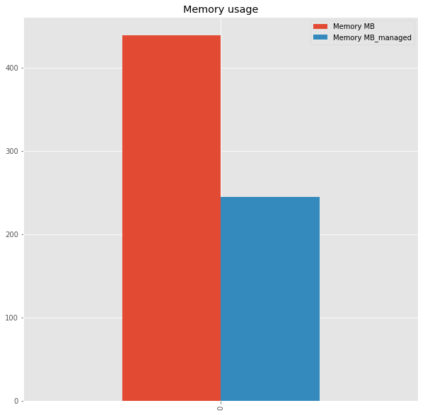
DataFrame Memory MB DataFrame_managed Memory MB_managed
0 processed_user_log 439.264153 processed_user_log 244.590301
With the right type for each feature, we have reduced the usage by 44%. It is not negligible especially when we have a constraint on the hardware or when you need your the memory to implement a machine learning model. It exists others methods to reduce the memory usage. You have to be careful on the type of each feature if you want to optimize the manipulation of the data.
Post comment below if you have questions.
nice postpython training in chennai
Very interesting post! Thanks for sharing!
Intriguing post. I definitely learned something here. I would also suggest using built in functions to access, read, and bring in data from files instead of using the Pandas library, if saving memory and speed is a higher goal.
Hi, nice post! But how do you get the 7z compressed file into python from the link you shared. Or do you have it already stored on your machine?
Hi, great post!
I have a doubt, why not use a sql for doing this aggregations? it will require only one process to get the results.
Rgds